Getting Started

• 1: Installation
• 2: Site Organisation
• 3: Getting Help
• 4: Your First Project

(ql:quickload :lisp-stat)
(in-package :ls-user)     ;access to Lisp-Stat functions

(ql:quickload :plot/vega)

(data :vgcars)

(print-data vgcars)
;; ORIGIN YEAR       ACCELERATION WEIGHT_IN_LBS HORSEPOWER DISPLACEMENT CYLINDERS MILES_PER_GALLON NAME
;; USA    1970-01-01         12.0          3504        130        307.0         8             18.0 chevrolet chevelle malibu
;; USA    1970-01-01         11.5          3693        165        350.0         8             15.0 buick skylark 320
;; USA    1970-01-01         11.0          3436        150        318.0         8             18.0 plymouth satellite
;; USA    1970-01-01         12.0          3433        150        304.0         8             16.0 amc rebel sst
;; USA    1970-01-01         10.5          3449        140        302.0         8             17.0 ford torino
;; USA    1970-01-01         10.0          4341        198        429.0         8             15.0 ford galaxie 500
;; USA    1970-01-01          9.0          4354        220        454.0         8             14.0 chevrolet impala
;; USA    1970-01-01          8.5          4312        215        440.0         8             14.0 plymouth fury iii
;; USA    1970-01-01         10.0          4425        225        455.0         8             14.0 pontiac catalina
;; USA    1970-01-01          8.5          3850        190        390.0         8             15.0 amc ambassador dpl
;; Europe 1970-01-01         17.5          3090        115        133.0         4 NIL              citroen ds-21 pallas
;; USA    1970-01-01         11.5          4142        165        350.0         8 NIL              chevrolet chevelle concours (sw)
;; USA    1970-01-01         11.0          4034        153        351.0         8 NIL              ford torino (sw)
;; USA    1970-01-01         10.5          4166        175        383.0         8 NIL              plymouth satellite (sw)
;; USA    1970-01-01         11.0          3850        175        360.0         8 NIL              amc rebel sst (sw)
;; USA    1970-01-01         10.0          3563        170        383.0         8             15.0 dodge challenger se
;; USA    1970-01-01          8.0          3609        160        340.0         8             14.0 plymouth 'cuda 340
;; USA    1970-01-01          8.0          3353        140        302.0         8 NIL              ford mustang boss 302
;; USA    1970-01-01          9.5          3761        150        400.0         8             15.0 chevrolet monte carlo
;; USA    1970-01-01         10.0          3086        225        455.0         8             14.0 buick estate wagon (sw)
;; Japan  1970-01-01         15.0          2372         95        113.0         4             24.0 toyota corona mark ii
;; USA    1970-01-01         15.5          2833         95        198.0         6             22.0 plymouth duster
;; USA    1970-01-01         15.5          2774         97        199.0         6             18.0 amc hornet
;; USA    1970-01-01         16.0          2587         85        200.0         6             21.0 ford maverick                 ..

(tail vgcars)
;; ORIGIN YEAR       ACCELERATION WEIGHT_IN_LBS HORSEPOWER DISPLACEMENT CYLINDERS MILES_PER_GALLON NAME
;; USA    1982-01-01         17.3          2950         90          151         4               27 chevrolet camaro
;; USA    1982-01-01         15.6          2790         86          140         4               27 ford mustang gl
;; Europe 1982-01-01         24.6          2130         52           97         4               44 vw pickup
;; USA    1982-01-01         11.6          2295         84          135         4               32 dodge rampage
;; USA    1982-01-01         18.6          2625         79          120         4               28 ford ranger
;; USA    1982-01-01         19.4          2720         82          119         4               31 chevy s-10

(mean vgcars:acceleration) ; => 15.5197

LS-USER> (summary vgcars)

"ORIGIN": 254 (63%) x "USA", 79 (19%) x "Japan", 73 (18%) x "Europe"

"YEAR": 61 (15%) x "1982-01-01", 40 (10%) x "1973-01-01", 36 (9%) x "1978-01-01", 35 (9%) x "1970-01-01", 34 (8%) x "1976-01-01", 30 (7%) x "1975-01-01", 29 (7%) x "1971-01-01", 29 (7%) x "1979-01-01", 29 (7%) x "1980-01-01", 28 (7%) x "1972-01-01", 28 (7%) x "1977-01-01", 27 (7%) x "1974-01-01"

ACCELERATION (1/4 mile time)
 n: 406
 missing: 0
 min=8
 q25=13.67
 q50=15.45
 mean=15.52
 q75=17.17
 max=24.80

WEIGHT-IN-LBS (Weight in lbs)
 n: 406
 missing: 0
 min=1613
 q25=2226
 q50=2822.50
 mean=2979.41
 q75=3620
 max=5140
...

(plot:plot
  (vega:defplot hp-mpg
    `(:title "Horsepower vs. MPG"
      :description "Horsepower vs miles per gallon for various cars"
      :data (:values ,vgcars)
      :mark :point
      :encoding (:x (:field :horsepower :type :quantitative)
	             :y (:field :miles-per-gallon :type :quantitative)))))

1 - Installation

Notebook

The easiest way to get started is with the link above which will open a preconfigured notebook on mybinder.org.

Users new to lisp should also consider going through the Lisp-Stat basic tutorial, which guides you step-by-step through the basics of working with Lisp as a statistics practitioner.

OCI/Docker

You can also run a pre-built OCI image. This is a minimal Docker file:

FROM ghcr.io/lisp-stat/cl-jupyter:latest

Our images are based on Jupyter Docker Stacks and all of their documentation is applicable to the cl-jupyter image.

For a quickstart:

docker run -it -p 8888:8888 ghcr.io/lisp-stat/cl-jupyter:latest

# Entered start.sh with args: jupyter lab

# ...

#     To access the server, open this file in a browser:
#         file:///home/jovyan/.local/share/jupyter/runtime/jpserver-7-open.html
#     Or copy and paste one of these URLs:
#         http://eca4aa01751c:8888/lab?token=d4ac9278f5f5388e88097a3a8ebbe9401be206cfa0b83099
#         http://127.0.0.1:8888/lab?token=d4ac9278f5f5388e88097a3a8ebbe9401be206cfa0b83099

This command pulls the latest cl-jupyter image from ghcr.io if it is not already present on the local host. It then starts a container running a Jupyter Server with the JupyterLab frontend and exposes the server on host port 8888. The server logs appear in the terminal and include a URL to the server.

Initialization file

You can put customisations to your environment in either your implementation’s init file, or in a personal init file and load it from the implementation’s init file. For example, I keep my customisations in #P"~/ls-init.lisp" and load it from SBCL’s init file ~/.sbclrc in a Lisp-Stat initialisation section like this:

;;; Lisp-Stat
(asdf:load-system :lisp-stat)
(load #P"~/ls-init.lisp")

Settings in your personal lisp-stat init file override the system defaults.

Here’s an example ls-init.lisp file that loads some common R data sets:

(defparameter *default-datasets*
  '("tooth-growth" "plant-growth" "usarrests" "iris" "mtcars")
  "Data sets loaded as part of personal Lisp-Stat initialisation.
  Available in every session.")

(map nil #'(lambda (x)
	     (format t "Loading ~A~%" x)
	     (data x))
	     *default-datasets*)

With this init file, you can immediately access the data sets in the *default-datasets* list defined above, e.g.:

(head iris)
;;   X2 SEPAL-LENGTH SEPAL-WIDTH PETAL-LENGTH PETAL-WIDTH SPECIES
;; 0  1          5.1         3.5          1.4         0.2 setosa
;; 1  2          4.9         3.0          1.4         0.2 setosa
;; 2  3          4.7         3.2          1.3         0.2 setosa
;; 3  4          4.6         3.1          1.5         0.2 setosa
;; 4  5          5.0         3.6          1.4         0.2 setosa
;; 5  6          5.4         3.9          1.7         0.4 setosa

Emacs / Hemlock

We assume an experienced user will have their own Emacs and lisp implementation and will want to install according to their own tastes and setup. The repo links you need are below, or you can install with quicklisp.

Prerequisites

All that is needed is an ANSI Common Lisp implementation. Development is done with SBCL. Other platforms should work, but will not have been tested, nor can we offer support (maintaining & testing on multiple implementations requires more resources than the project has available). Note that CCL is not in good health, and there are a few numerical bugs that remain unfixed. A shame, as we really liked CCL.

You may want to consider emacs-vega-view for viewing plots from within emacs.

Installation

The easiest way to install Lisp-Stat is via Quicklisp, a library manager for Common Lisp. It works with your existing Common Lisp implementation to download, install, and load any of over 1,500 libraries with a few simple commands.

Quicklisp is like a package manager in Linux. It can load packages from the local file system, or download them if required. If you have quicklisp installed, you can use:

(ql:quickload :lisp-stat)

Quicklisp is good at managing the project dependency retrieval, but most of the time we use ASDF because of its REPL integration. You only have to use Quicklisp once to get the dependencies, then use ASDF for day-to-day work.

You can install additional Lisp-Stat modules in the same way. For example to install the CEPHES module:

(ql:quickload :cephes)

Loading

Once you have obtained Lisp-Stat via Quicklisp, you can load in one of two ways:

• ASDF
• Quicklisp

Loading with ASDF

(asdf:load-system :lisp-stat)

If you are using emacs, you can use the slime shortcuts to load systems by typing , and then load-system in the mini-buffer. This is what the Lisp-Stat developers use most often, the shortcuts are a helpful part of the workflow.

Loading with Quicklisp

To load with Quicklisp:

(ql:quickload :lisp-stat)

Quicklisp uses the same ASDF command as above to load Lisp-Stat.

Updating Lisp-Stat

When a new release is announced, you can update via Quicklisp like so:

(ql:update-dist "lisp-stat")

Documentation

You can install the info manuals into the emacs help system and this allows searching and browsing from within the editing environment. To do this, use the install-info command. As an example, on my MS Windows 10 machine, with MSYS2/emacs installation:

install-info --add-once select.info /c/msys64/mingw64/share/info/dir

installs the select manual at the top level of the info tree. You can also install the common lisp hyperspec and browse documentation for the base Common Lisp system. This really is the best way to use documentation whilst programming Common Lisp and Lisp-Stat. See the emacs external documentation and “How do I install a piece of Texinfo documentation?” for more information on installing help files in emacs.

See getting help for information on how to access Info documentation as you code. This is the mechanism used by Lisp-Stat developers because you don’t have to leave the emacs editor to look up function documentation in a browser.

Try it out

Load Lisp-Stat:

(asdf:load-system :lisp-stat)

Change to the Lisp-Stat user package:

(in-package :ls-user)

Load some data:

(data :sg-weather)

Find the sample mean and median:

(mean sg-weather:precipitation) ;=> .0714
(median sg-weather:max-temps)   ;=> 31.55

Next steps

2 - Site Organisation

This manual is organised by audience. The overview and getting started sections are applicable to all users. Other sections are focused on statistical practitioners, developers or users new to Common Lisp.

Examples

This part of the documentation contains worked examples of statistical analysis and plotting. It has less explanatory material, and more worked examples of code than other sections. If you have a common use-case and want to know how to solve it, look here.

Tutorials

This section contains tutorials, primers and ‘vignettes’. Typically tutorials contain more explanatory material, whilst primers are short-form tutorials on a particular system.

System manuals

The manuals are written at a level somewhere between an API reference and a core task. (‘annotated reference’) They document, with text and examples, the core APIs of each system. These are useful references for power users, developers and if you need to go a bit beyond the core tasks.

Reference

The reference manuals document the API for each system. These are typically used by developers building extensions to Lisp-Stat.

Resources

Common Lisp and statistical resources, such as books, tutorials and website. Not specific to Lisp-Stat, but useful for statistical practitioners learning Lisp.

Contributing

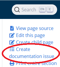
This section describes how to contribute to Lisp-Stat. There are both ideas on what to contribute, as well as instructions on how to contribute. Also note the section on the top right of all the documentation pages, just below the search box:

If you see a mistake in the documentation, please use the Create documentation issue link to go directly to github and report the error.

3 - Getting Help

There are several ways to get help with Lisp-Stat and your statistical analysis. This section describes way to get help with your data objects, with Lisp-Stat commands to process them, and with Common Lisp.

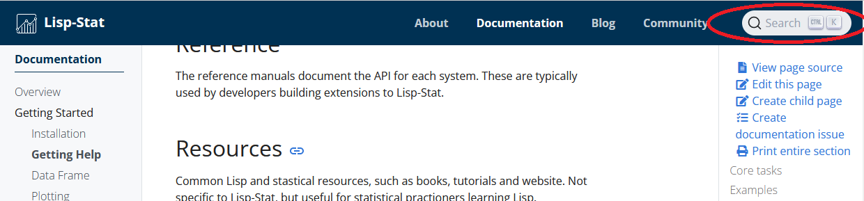
Search

We use the algolia search engine to index the site. This search engine is specialised to work well with documentation websites like this one. If you’re looking for something and can’t find it in the navigation panes, use the search box:

Apropos

If you’re not quite sure what you’re looking for, you can use the apropos command. You can do this either from the REPL or hemlock/emacs. Here are two examples:

LS-USER> (apropos "remove-if")
SB-SEQUENCE:REMOVE-IF (fbound)
SB-SEQUENCE:REMOVE-IF-NOT (fbound)
REMOVE-IF (fbound)
REMOVE-IF-NOT (fbound)

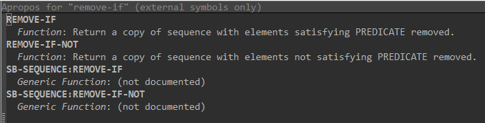
If you use the emacs/slime command sequence C-c C-d a, (all the slime documentation commands start with C-c C-d) emacs will ask you for a string. Let’s say you typed in remove-if. Emacs will open a buffer like the one below with all the docs strings for similar functions or variables:

Restart from errors

Common lisp has what is called a condition system, which is somewhat unique. One of the features of the condition system is something call restarts. Basically, one part of the system can signal a condition, and another part of it can handle the condition. One of the ways a signal can be handled is by providing various restarts. Restarts happen by the debugger, and many users new to Common Lisp tend to shy away from the debugger (this is common to other languages too). In Common Lisp the debugger is both for developers and users.

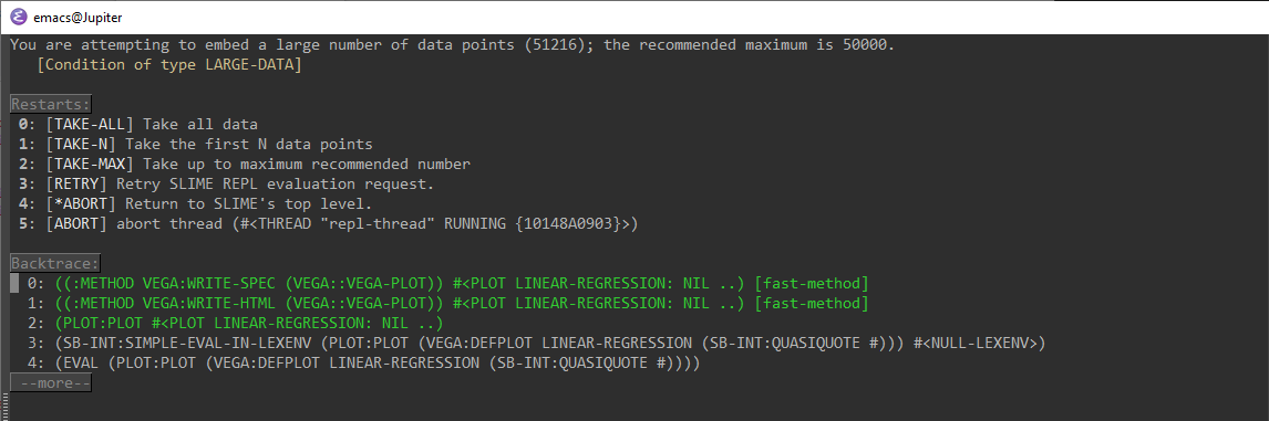
Well written Lisp programs will provide a good set of restarts for commonly encountered situations. As an example, suppose we are plotting a data set that has a large number of data points. Experience has shown that greater than 50,000 data points can cause browser performance issues, so we’ve added a restart to warn you, seen below:

Here you can see we have options to take all the data, take n (that the user will provide) or take up to the maximum recommended number. Always look at the options offered to you by the debugger and see if any of them will fix the problem for you.

Describe data

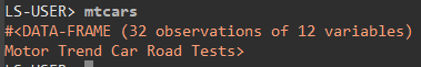
You can use the describe command to print a description of just about anything in the Lisp environment. Lisp-Stat extends this functionality to describe data. For example:

LS-USER> (describe 'mtcars)
LS-USER::MTCARS
  [symbol]

MTCARS names a special variable:
  Value: #<DATA-FRAME (32 observations of 12 variables)
Motor Trend Car Road Tests>
  Documentation:
    Motor Trend Car Road Tests

	Description
    The data was extracted from the 1974 Motor Trend US magazine, and
	comprises fuel consumption and 10 aspects of automobile design and
	performance for 32 automobiles (1973–74 models).

    Note
    Henderson and Velleman (1981) comment in a footnote to Table 1:
	‘Hocking [original transcriber]'s noncrucial coding of the Mazda's
	rotary engine as a straight six-cylinder engine and the Porsche's
	flat engine as a V engine, as well as the inclusion of the diesel
	Mercedes 240D, have been retained to enable direct comparisons to
	be made with previous analyses.’

    Source
    Henderson and Velleman (1981), Building multiple regression models
	interactively. Biometrics, 37, 391–411.

  Variables:
    Variable | Type         | Unit | Label
    -------- | ----         | ---- | -----------
    MODEL    | STRING       | NIL  | NIL
    MPG      | DOUBLE-FLOAT | M/G  | Miles/(US) gallon
    CYL      | INTEGER      | NA   | Number of cylinders
    DISP     | DOUBLE-FLOAT | IN3  | Displacement (cu.in.)
    HP       | INTEGER      | HP   | Gross horsepower
    DRAT     | DOUBLE-FLOAT | NA   | Rear axle ratio
    WT       | DOUBLE-FLOAT | LB   | Weight (1000 lbs)
    QSEC     | DOUBLE-FLOAT | S    | 1/4 mile time
    VS       | CATEGORICAL  | NA   | Engine (0=v-shaped, 1=straight)
    AM       | CATEGORICAL  | NA   | Transmission (0=automatic, 1=manual)
    GEAR     | CATEGORICAL  | NA   | Number of forward gears
    CARB     | CATEGORICAL  | NA   | Number of carburetors

Documentation

The documentation command can be used to read the documentation of a function or variable. Here’s how to read the documentation for the Lisp-Stat mean function:

LS-USER> (documentation 'mean 'function)
"The mean of elements in OBJECT."

You can also view the documentation for variables or data objects:

LS-USER> (documentation '*ask-on-redefine* 'variable)

"If non-nil the system will ask the user for confirmation
before redefining a data frame"

Emacs inspector

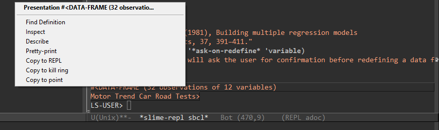
When Lisp prints an interesting object to emacs/slime, it will be displayed in orange text. This indicates that it is a presentation, a special kind of object that we can manipulate. For example if you type the name of a data frame, it will return a presentation object:

Now if you right click on this object you’ll get the presentation menu:

From this menu you can go to the source code of the object, inspect & change values, describe it (as seen above, but within an emacs window), and copy it.

Slime inspector

The slime inspector is an alternative inspector for emacs, with some additional functionality.

Slime documentation

Slime documentation provides ways to browse documentation from the editor. We saw one example above with apropos. You can also browse variable and function documentation. For example if you have the cursor positioned over a function:

(show-data-frames)

and you type C-c C-d f (describe function at point), you’ll see this in an emacs window:

#<FUNCTION SHOW-DATA-FRAMES>
  [compiled function]


Lambda-list: (&KEY (HEAD NIL) (STREAM *STANDARD-OUTPUT*))
Derived type: (FUNCTION (&KEY (:HEAD T) (:STREAM T)) *)
Documentation:
  Print all data frames in the current environment in
  reverse order of creation, i.e. most recently created first.
  If HEAD is not NIL, print the first six rows, similar to the
  HEAD function.
Source file: s:/src/data-frame/src/defdf.lisp

Other help

You can also get help from the Lisp-Stat community, the user mailing list, github or stackoverflow

4 - Your First Project

Lisp-Stat includes a project template that you can use as a guide for your own projects.

Use the template

To get started, go to the project template

1. Click Use this template
2. Select a name for your new project and click Create repository from template
3. Make your own local working copy of your new repo using git clone, replacing https://github.com/me/example.git with your repo’s URL: git clone --depth 1 https://github.com/me/example.git
4. You can now edit your own versions of the project’s source files.

This will clone the project template into your own github repository so you can begin adding your own files to it.

Directory Structure

By convention, we use a directory structure that looks like this:

...
├── project
|   ├── data
|   |   ├── foo.csv
|   |   ├── bar.json
|   |   └── baz.tsv
|   └── src
|   |   ├── load.lisp
|   |   └── analyse.lisp
|   |   └── baz.tsv
|   └── tests
|   |   ├── test.lisp
|   └── doc
|   |   ├── project.html
...

data

Often your project will have sample data used for examples illustrating how to use the system. Such example data goes here, as would static data files that your system includes, for example post codes (zip codes). For some projects, we keep the project data here too. If the data is obtained over the network or a data base, login credentials and code related to that is kept here. Basically, anything neccessary to obtain the data should be kept in this directory.

src

The lisp source code for loading, cleaning and analysing your data. If you are using the template for a Lisp-Stat add-on package, the source code for the functionality goes here.

tests

Tests for your code. We recommend CL-UNIT2 for test frameworks.

docs

Generated documentation goes here. This could be both API documentation and user guides and manuals. If an index.html file appears here, github will automatically display it’s contents at project.github.io, if you have configured the repository to display documentation that way.

Load your project

If you’ve cloned the project template into your local Common Lisp directory, ~/common-lisp/, then you can load it with (ql:quickload :project). Lisp will download and compile the necessary dependencies and your project will be loaded. The first thing you’ll want to do is to configure your project.

Configure your project

First, change the directory and repository name to suit your environment and make sure git remotes are working properly. Save yourself some time and get git working before configuring the project further.

ASDF

The project.asd file is the Common Lisp system definition file. Rename this to be the same as your project directory and edit its contents to reflect the state of your project. To start with, don’t change any of the file names; just edit the meta data. As you add or rename source code files in the project you’ll update the file names here so Common Lisp will know that to compile. This file is analgous to a makefile in C – it tells lisp how to build your project.

Initialisation

If you need project-wide initialisation settings, you can do this in the file src/init.lisp. The template sets up a logical path name for the project:

(defun setup-project-translations ()
  (setf (logical-pathname-translations "PROJECT")
	`(("DATA;**;*.*.*"    ,(merge-pathnames "data/**/*.*" (asdf:system-source-directory 'project))))))

(setup-project-translations)

To use it, you’ll modify the directories and project name for your project, and then call (setup-project-translations) in one of your lisp initialisation files (either ls-init.lisp or .sbclrc). By default, the project data directory will be set to a subdirectory below the main project directory, and you can access files there with PROJECT:DATA;mtcars.csv for example. When you configure your logical pathnames, you’ll replace “PROJECT” with your projects name.

We use logical style pathnames throughout the Lisp-Stat documentation, even if a code level translation isn’t in place.

Basic workflow

The project templates illustrates the basic steps for a simple analysis.

Load data

The first step is to load data. The PROJECT:SRC;load file shows creating three data frames, from three different sources: CSV, TSV and JSON. Use this as a template for loading your own data.

Cleanse data

load.lisp also shows some simple cleansing, adding labels, types and attributes, and transforming (recoding) a variable. You can follow these examples for your own data sets, with the goal of creating a data frame from your data.

Analyse

PROJECT:SRC;analyse shows taking the mean and standard deviation of the mpg variable of the loaded data set. Your own analysis will, of course, be different. The examples here are meant to indicate the purpose. You may have one or more files for your analysis, including supporting functions, joining data sets, etc.

Plot

Plotting can be useful at any stage of the process. It’s inclusion as the third step isn’t intended to imply a particular importance or order. The file PROJECT:SRC;plot shows how to plot the information in the disasters data frame.

Save

Finally, you’ll want to save your data frame after you’ve got it where you want it to be. You can save project in a ’native’ format, a lisp file, that will preserve all your meta data and is editable, or a CSV file. You should only use a CSV file if you need to use the data in another system. PROJECT:SRC;save containes an example that shows how to save your work.