This section describes the core APIs and systems that comprise Lisp-Stat. These APIs include both the high level functionality described elsewhere, as well as lower level APIs that they are built on. This section will be of interest to ‘power users’ and developers who wish to extend Lisp-Stat, or build modules of their own.
This is the multi-page printable view of this section. Click here to print.
System Manuals
Manuals for Lisp-Stat systems
- 1: Array Operations
- 2: Data Frame
- 3: Distributions
- 4: Numeric Utilities
- 5: Linear Algebra
- 6: Select
- 7: SQLDF
- 8: Statistics
1 - Array Operations
Manipulating sample data as arrays
Overview
The array-operations system contains a collection of functions and
macros for manipulating Common Lisp arrays and performing numerical
calculations with them.
Array-operations is a ‘generic’ way of operating on array like data
structures. Several aops functions have been implemented for
data-frame. For those that haven’t, you can transform arrays to
data frames using the df:matrix-df function, and a data-frame to an
array using df:as-array. This make it convenient to work with the
data sets using either system.
Quick look
Arrays can be created with numbers from a statistical distribution:
(rand '(2 2)) ; => #2A((0.62944734 0.2709539) (0.81158376 0.6700171))
in linear ranges:
(linspace 1 10 7) ; => #(1 5/2 4 11/2 7 17/2 10)
or generated using a function, optionally given index position
(generate #'identity '(2 3) :position) ; => #2A((0 1 2) (3 4 5))
They can also be transformed and manipulated:
(defparameter A #2A((1 2)
                    (3 4)))
(defparameter B #2A((2 3)
                    (4 5)))

;; split along any dimension
(split A 1)  ; => #(#(1 2) #(3 4))

;; stack along any dimension
(stack 1 A B) ; => #2A((1 2 2 3)
              ;        (3 4 4 5))

;; element-wise function map
(each #'+ #(0 1 2) #(2 3 5)) ; => #(2 4 7)

;; element-wise expressions
(vectorize (A B) (* A (sqrt B))) ; => #2A((1.4142135 3.4641016)
                                 ;        (6.0       8.944272))

;; index operations e.g. matrix-matrix multiply:
(each-index (i j)
  (sum-index k
    (* (aref A i k) (aref B k j)))) ; => #2A((10 13)
	                                ;        (22 29))
Array shorthand
The library defines the following short function names that are synonyms for Common Lisp operations:
| array-operations | Common Lisp |
|---|---|
| size | array-total-size |
| rank | array-rank |
| dim | array-dimension |
| dims | array-dimensions |
| nrow | number of rows in matrix |
| ncol | number of columns in matrix |
The array-operations package has the nickname aops, so you can use,
for example, (aops:size my-array) without use‘ing the package.
Displaced arrays
According to the Common Lisp specification, a displaced array is:
An array which has no storage of its own, but which is instead indirected to the storage of another array, called its target, at a specified offset, in such a way that any attempt to access the displaced array implicitly references the target array.
Displaced arrays are one of the niftiest features of Common Lisp. When an array is displaced to another array, it shares structure with (part of) that array. The two arrays do not need to have the same dimensions, in fact, the dimensions do not be related at all as long as the displaced array fits inside the original one. The row-major index of the former in the latter is called the offset of the displacement.
displace
Displaced arrays are usually constructed using make-array, but this
library also provides displace for that purpose:
(defparameter *a* #2A((1 2 3)
                      (4 5 6)))
(aops:displace *a* 2 1) ; => #(2 3)
Here’s an example of using displace to implement a sliding window over some set of values, say perhaps a time-series of stock prices:
(defparameter stocks (aops:linspace 1 100 100))
(loop for i from 0 to (- (length stocks) 20)
      do (format t "~A~%" (aops:displace stocks 20 i)))
;#(1 2 3 4 5 6 7 8 9 10 11 12 13 14 15 16 17 18 19 20)
;#(2 3 4 5 6 7 8 9 10 11 12 13 14 15 16 17 18 19 20 21)
;#(3 4 5 6 7 8 9 10 11 12 13 14 15 16 17 18 19 20 21 22)
flatten
flatten displaces to a row-major array:
(aops:flatten *a*) ; => #(1 2 3 4 5 6)
split
The real fun starts with split, which splits off sub-arrays nested
within a given axis:
(aops:split *a* 1) ; => #(#(1 2 3) #(4 5 6))
(defparameter *b* #3A(((0 1) (2 3))
                      ((4 5) (6 7))))
(aops:split *b* 0) ; => #3A(((0 1) (2 3)) ((4 5) (6 7)))
(aops:split *b* 1) ; => #(#2A((0 1) (2 3)) #2A((4 5) (6 7)))
(aops:split *b* 2) ; => #2A((#(0 1) #(2 3)) (#(4 5) #(6 7)))
(aops:split *b* 3) ; => #3A(((0 1) (2 3)) ((4 5) (6 7)))
Note how splitting at 0 and the rank of the array returns the array
itself.
sub
Now consider sub, which returns a specific array, composed of the
elements that would start with given subscripts:
(aops:sub *b* 0) ; => #2A((0 1)
                 ;        (2 3))
(aops:sub *b* 0 1) ; => #(2 3)
(aops:sub *b* 0 1 0) ; => 2
In the case of vectors, sub works like aref:
(aops:sub #(1 2 3 4 5) 1) ; => 2
There is also a (setf sub) function.
partition
partition returns a consecutive chunk of an array separated along its
first subscript:
(aops:partition #2A((0 1)
                    (2 3)
                    (4 5)
                    (6 7)
                    (8 9))
              1 3) ; => #2A((2 3)
			       ;        (4 5))
and also has a (setf partition) pair.
combine
combine is the opposite of split:
(aops:combine #(#(0 1) #(2 3))) ; => #2A((0 1)
                                ;        (2 3))
subvec
subvec returns a displaced subvector:
(aops:subvec #(0 1 2 3 4) 2 4) ; => #(2 3)
There is also a (setf subvec) function, which is like (setf subseq)
except for demanding matching lengths.
reshape
Finally, reshape can be used to displace arrays into a different
shape:
(aops:reshape #2A((1 2 3)
                  (4 5 6)) '(3 2))
; => #2A((1 2)
;        (3 4)
;        (5 6))
You can use t for one of the dimensions, to be filled in
automatically:
(aops:reshape *b* '(1 t)) ; => #2A((0 1 2 3 4 5 6 7))
reshape-col and reshape-row reshape your array into a column or row
matrix, respectively:
(defparameter *a* #2A((0 1)
                      (2 3)
					  (4 5)))
(aops:reshape-row *a*) ;=> #2A((0 1 2 3 4 5))
(aops:reshape-col *a*) ;=> #2A((0) (1) (2) (3) (4) (5))
Specifying dimensions
Functions in the library accept the following in place of dimensions:
- a list of dimensions (as for
make-array), - a positive integer, which is used as a single-element list,
- another array, the dimensions of which are used.
The last one allows you to specify dimensions with other arrays. For
example, to reshape an array a1 to look like a2, you can use
(aops:reshape a1 a2)
instead of the longer form
(aops:reshape a1 (aops:dims a2))
Creation & transformation
Use the functions in this section to create commonly used arrays
types. When the resulting element type cannot be inferred from an
existing array or vector, you can pass the element type as an optional
argument. The default is elements of type T.
Element traversal order of these functions is unspecified. The reason for this is that the library may use parallel code in the future, so it is unsafe to rely on a particular element traversal order.
The following functions all make a new array, taking the dimensions as
input. There are also versions ending in ! which do not make a
new array, but take an array as first argument, which is modified and
returned.
| Function | Description |
|---|---|
| zeros | Filled with zeros |
| ones | Filled with ones |
| rand | Filled with uniformly distributed random numbers between 0 and 1 |
| randn | Normally distributed with mean 0 and standard deviation 1 |
| linspace | Evenly spaced numbers in given range |
For example:
(aops:zeros 3)
; => #(0 0 0)

(aops:zeros 3 'double-float)
; => #(0.0d0 0.0d0 0.0d0)

(aops:rand '(2 2))
; => #2A((0.6686077 0.59425664)
;        (0.7987722 0.6930506))

(aops:rand '(2 2) 'single-float)
; => #2A((0.39332366 0.5557821)
;        (0.48831415 0.10924244))

(let ((a (make-array '(2 2) :element-type 'double-float)))
  ;; Modify array A, filling with random numbers
  ;; element type is taken from existing array
  (aops:rand! a))
  ; => #2A((0.6324615478515625d0 0.4636608362197876d0)
  ;        (0.4145939350128174d0 0.5124958753585815d0))
(linspace 0 4 5)   ;=> #(0 1 2 3 4)
(linspace 1 3 5)   ;=> #(0 1/2 1 3/2 2)
(linspace 1 3 5 'double-float) ;=> #(1.0d0 1.5d0 2.0d0 2.5d0 3.0d0)
(linspace 0 4d0 3) ;=> #(0.0d0 2.0d0 4.0d0)
generate
generate (and generate*) allow you to generate arrays using
functions. The function signatures are:
generate* (element-type function dimensions &optional arguments)
generate (function dimensions &optional arguments)
Where arguments are passed to function. Possible arguments are:
- no arguments, when ARGUMENTS is nil
- the position (= row major index), when ARGUMENTS is :POSITION
- a list of subscripts, when ARGUMENTS is :SUBSCRIPTS
- both when ARGUMENTS is :POSITION-AND-SUBSCRIPTS
(aops:generate (lambda () (random 10)) 3) ; => #(6 9 5)

(aops:generate #'identity '(2 3) :position) ; => #2A((0 1 2)
                                            ;        (3 4 5))

(aops:generate #'identity '(2 2) :subscripts)
; => #2A(((0 0) (0 1))
;        ((1 0) (1 1)))

(aops:generate #'cons '(2 2) :position-and-subscripts)
; => #2A(((0 0 0) (1 0 1))
;        ((2 1 0) (3 1 1)))
permute
permute can permute subscripts (you can also invert, complement, and
complete permutations, look at the docstring and the unit tests).
Transposing is a special case of permute:
(defparameter *a* #2A((1 2 3)
                      (4 5 6)))
(aops:permute '(0 1) *a*) ; => #2A((1 2 3)
                          ;        (4 5 6))
(aops:permute '(1 0) *a*) ; => #2A((1 4)
                          ;        (2 5)
						  ;        (3 6))
each
each applies a function to its one dimensional array arguments
elementwise. It essentially is an element-wise function map on each of
the vectors:
(aops:each #'+ #(0 1 2)
               #(2 3 5)
			   #(1 1 1)
; => #(3 5 8)
vectorize
vectorize is a macro which performs elementwise operations
(defparameter a #(1 2 3 4))
(aops:vectorize (a) (* 2 a)) ; => #(2 4 6 8)

(defparameter b #(2 3 4 5))
(aops:vectorize (a b) (* a (sin b)))
; => #(0.9092974 0.28224 -2.2704074 -3.8356972)
There is also a version vectorize* which takes a type argument for the
resulting array, and a version vectorize! which sets elements in a
given array.
margin
The semantics of margin are more difficult to explain, so perhaps an
example will be more useful. Suppose that you want to calculate column
sums in a matrix. You could permute (transpose) the matrix, split
its sub-arrays at rank one (so you get a vector for each row), and apply
the function that calculates the sum. margin automates that for you:
(aops:margin (lambda (column)
               (reduce #'+ column))
           #2A((0 1)
               (2 3)
               (5 7)) 0) ; => #(7 11)
But the function is more general than this: the arguments inner and
outer allow arbitrary permutations before splitting.
recycle
Finally, recycle allows you to reuse the elements of the first argument, object, to create new arrays by extending the dimensions. The :outer keyword repeats the original object and :inner keyword argument repeats the elements of object. When both :inner and :outer are nil, object is returned as is. Non-array objects are intepreted as rank 0 arrays, following the usual semantics.
(aops:recycle #(2 3) :inner 2 :outer 4)
; => #3A(((2 2) (3 3))
         ((2 2) (3 3))
         ((2 2) (3 3))
	     ((2 2) (3 3)))
Three dimensional arrays can be tough to get your head around. In the example above, :outer asks for 4 2-element vectors, composed of repeating the elements of object twice, i.e. repeat ‘2’ twice and repeat ‘3’ twice. Compare this with :inner as 3:
(aops:recycle #(2 3) :inner 3 :outer 4)
; #3A(((2 2 2) (3 3 3))
      ((2 2 2) (3 3 3))
	  ((2 2 2) (3 3 3))
	  ((2 2 2) (3 3 3)))
The most common use case for recycle is to ‘stretch’ a vector so that it can be an operand for an array of compatible dimensions. In Python, this would be known as ‘broadcasting’. See the Numpy broadcasting basics for other use cases.
For example, suppose we wish to multiply array a, of size 4x3, with vector b, of size 1x3, as in the figure below:
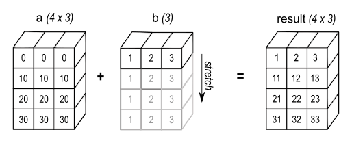
We can do that by recycling array b like this:
(recycle #(1 2 3) :outer 4)
;#2A((1 2 3)
;	 (1 2 3)
;	 (1 2 3)
;	 (1 2 3))
In a similar manner, the figure below (also from the Numpy page) shows how we might stretch a vector horizontally to create an array compatible with the one created above.
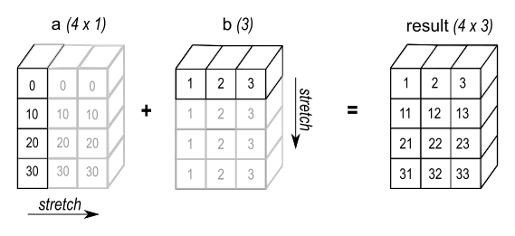
To create that array from a vector, use the :inner keyword:
(recycle #(0 10 20 30) :inner 3)
;#2A((0 0 0)
;	 (10 10 10)
;	 (20 20 20)
;	 (30 30 30))
turn
turn rotates an array by a specified number of clockwise 90° rotations. The axis of rotation is specified by RANK-1 (defaulting to 0) and RANK-2 (defaulting to 1). In the first example, we’ll rotate by 90°:
(defparameter array-1 #2A((1 0 0)
                          (2 0 0)
                          (3 0 0)))
(aops:turn array-1 1)
;; #2A((3 2 1)
;;     (0 0 0)
;;	   (0 0 0))
and if we rotate it twice (180°):
(aops:turn array-1 2)
;; #2A((0 0 3)
;;     (0 0 2)
;;     (0 0 1))
finally, rotate it three times (270°):
(aops:turn array-1 3)
;; #2A((0 0 0)
;;     (0 0 0)
;;     (1 2 3))
map-array
map-array maps a function over the elements of an array.
(aops:map-array #2A((1.7 2.1 4.3 5.4)
                    (0.3 0.4 0.5 0.6))
				#'log)
; #2A(( 0.53062826 0.7419373  1.4586151  1.686399)
;     (-1.2039728 -0.9162907 -0.6931472 -0.5108256))
outer
outer is generalized outer product of arrays using a provided function.
Lambda list: (function &rest arrays)
The resulting array has the concatenated dimensions of arrays
The examples below return the outer product of vectors or arrays. This is the outer product you get in most linear algebra packages.
(defparameter a #(2 3 5))
(defparameter b #(7 11))
(defparameter c #2A((7 11)
                    (13 17)))

(outer #'* a b)
;#2A((14 22)
;    (21 33)
;    (35 55))

(outer #'* c a)
;#3A(((14 21 35) (22 33 55))
;    ((26 39 65) (34 51 85)))
Indexing operations
sum-index
sum-index is a macro which uses a code walker to determine the
dimension sizes, summing over the given index or indices
(defparameter A #2A((1 2) (3 4)))

;; Trace
(aops:sum-index i (aref A i i)) ; => 5

;; Sum array
(aops:sum-index (i j) (aref A i j)) ; => 10

;; Sum array
(aops:sum-index i (row-major-aref A i)) ; => 10
The main use for sum-index is in combination with each-index.
each-index
each-index is a macro which creates an array and iterates over the
elements. Like sum-index it is given one or more index symbols, and
uses a code walker to find array dimensions.
(defparameter A #2A((1 2)
                    (3 4)))
(defparameter B #2A((5 6)
                    (7 8)))

;; Transpose
(aops:each-index (i j) (aref A j i)) ; => #2A((1 3)
                                     ;        (2 4))

;; Sum columns
(aops:each-index i
  (aops:sum-index j
    (aref A j i))) ; => #(4 6)

;; Matrix-matrix multiply
(aops:each-index (i j)
   (aops:sum-index k
      (* (aref A i k) (aref B k j)))) ; => #2A((19 22)
	                                  ;        (43 50))
reduce-index
reduce-index is a more general version of sum-index; it
applies a reduction operation over one or more indices.
(defparameter A #2A((1 2)
                    (3 4)))

;; Sum all values in an array
(aops:reduce-index #'+ i (row-major-aref A i)) ; => 10

;; Maximum value in each row
(aops:each-index i
  (aops:reduce-index #'max j
    (aref A i j)))  ; => #(2 4)
Reducing
Some reductions over array elements can be done using the Common Lisp
reduce function, together with aops:flatten, which returns a
displaced vector:
(defparameter a #2A((1 2)
                    (3 4)))
(reduce #'max (aops:flatten a)) ; => 4
argmax & argmin
argmax and argmin find the row-major-aref index where an
array value is maximum or minimum. They both return two values: the
first value is the index; the second is the array value at that index.
(defparameter a #(1 2 5 4 2))
(aops:argmax a) ; => 2 5
(aops:argmin a) ; => 0 1
vectorize-reduce
More complicated reductions can be done with vectorize-reduce,
for example the maximum absolute difference between arrays:
(defparameter a #2A((1 2)
                    (3 4)))
(defparameter b #2A((2 2)
                    (1 3)))

(aops:vectorize-reduce #'max (a b) (abs (- a b))) ; => 2
best
best compares two arrays according to a function and returns the ‘best’ value found. The function, FN must accept two inputs and return true/false. This function is applied to elements of ARRAY. The row-major-aref index is returned.
Example: The index of the maximum is
   * (best #'> #(1 2 3 4))
    3   ; row-major index
    4   ; value
most
most finds the element of ARRAY that returns the value closest to positive infinity when FN is applied to the array value. Returns the row-major-aref index, and the winning value.
Example: The maximum of an array is:
     (most #'identity #(1 2 3))
     -> 2    (row-major index)
        3    (value)
and the minimum of an array is:
      (most #'- #(1 2 3))
        0
        -1
See also reduce-index above.
Scalar values
Library functions treat non-array objects as if they were equivalent to
0-dimensional arrays: for example, (aops:split array (rank array))
returns an array that effectively equivalent (eq) to array. Another
example is recycle:
(aops:recycle 4 :inner '(2 2)) ; => #2A((4 4)
                               ;        (4 4))
Stacking
You can stack compatible arrays by column or row. Metaphorically you can think of these operations as stacking blocks. For example stacking two row vectors yields a 2x2 array:
(stack-rows #(1 2) #(3 4))
;; #2A((1 2)
;;     (3 4))
Like other functions, there are two versions: generalised stacking,
with rows and columns of type T and specialised versions where the
element-type is specified. The versions allowing you to specialise
the element type end in *.
The stack functions use object dimensions (as returned by dims to
determine how to use the object.
- when the object has 0 dimensions, fill a column with the element
- when the object has 1 dimension, use it as a column
- when the object has 2 dimensions, use it as a matrix
copy-row-major-block is a utility function in the stacking package
that does what it suggests; it copies elements from one array to
another. This function should be used to implement copying of
contiguous row-major blocks of elements.
rows
stack-rows-copy is the method used to implement the copying of objects in stack-row*, by copying the elements of source to destination, starting with the row index start-row in the latter. Elements are coerced to element-type.
stack-rows and stack-rows* stack objects row-wise into an array of the given element-type, coercing if necessary. Always return a simple array of rank 2. stack-rows always returns an array with elements of type T, stack-rows* coerces elements to the specified type.
columns
stack-cols-copy is a method used to implement the copying of objects in stack-col*, by copying the elements of source to destination, starting with the column index start-col in the latter. Elements are coerced to element-type.
stack-cols and stack-cols* stack objects column-wise into an array of the given element-type, coercing if necessary. Always return a simple array of rank 2. stack-cols always returns an array with elements of type T, stack-cols* coerces elements to the specified type.
arbitrary
stack and stack* stack array arguments along axis. element-type determines the element-type
of the result.
(defparameter *a1* #(0 1 2))
(defparameter *a2* #(3 5 7))
(aops:stack 0 *a1* *a2*) ; => #(0 1 2 3 5 7)
(aops:stack 1
          (aops:reshape-col *a1*)
          (aops:reshape-col *a2*)) ; => #2A((0 3)
	                               ;        (1 5)
								   ;        (2 7))
2 - Data Frame
Manipulating data using a data frame
Overview
A common lisp data frame is a collection of observations of sample variables that shares many of the properties of arrays and lists. By design it can be manipulated using the same mechanisms used to manipulate lisp arrays. This allow you to, for example, transform a data frame into an array and use array-operations to manipulate it, and then turn it into a data frame again to use in modeling or plotting.
Data frame is implemented as a two-dimensional common lisp data structure: a vector of vectors for data, and a hash table mapping variable names to column vectors. All columns are of equal length. This structure provides the flexibility required for column oriented manipulation, as well as speed for large data sets.
Note
In this document we refer to column and variable interchangeably. Likewise factor and category refer to a variable type. Where necessary we distinguish the terminology.Load/install
Data-frame is part of the Lisp-Stat package. It can be used independently if desired. Since the examples in this manual use Lisp-Stat functionality, we’ll use it from there rather than load independently.
(ql:quickload :lisp-stat)
Within the Lisp-Stat system, the LS-USER package is the package for
you to do statistics work. Type the following to change to that
package:
(in-package :ls-user)
Note
The examples assume that you are in package LS-USER. You should make a habit of always working from theLS-USER
package. All the samples may be copied to the clipboard using the
copy button in the upper-right corner of the sample code
box.
Naming conventions
Lisp-Stat has a few naming conventions you should be aware of. If you see a punctuation mark or the letter ‘p’ as the last letter of a function name, it indicates something about the function:
- ‘!’ indicates that the function is destructive. It will modify the data that you pass to it. Otherwise, it will return a copy that you will need to save in a variable.
- ‘p’, ‘-p’ or ‘?’ means the function is a predicate, that returns a Boolean truth value.
Data frame environment
Although you can work with data frames bound to symbols (as would
happen if you used (defparameter ...), it is more convenient to
define them as part of an environment. When you do this, the system
defines a package of the same name as the data frame, and provides a
symbol for each variable. Let’s see how things work without an
environment:
First, we define a data frame as a parameter:
(defparameter mtcars (read-csv rdata:mtcars)
"Motor Trend Car Road Tests")
;; WARNING: Missing column name was filled in
;; MTCARS2
Now if we want a column, we can say:
(column mtcars 'mpg)
Now let’s define an environment using defdf:
(defdf mtcars (read-csv rdata:mtcars)
"Motor Trend Car Road Tests")
;; WARNING: Missing column name was filled in
;; #<DATA-FRAME (32 observations of 12 variables)
;; Motor Trend Car Road Tests>
Now we can access the same variable with:
mtcars:mpg
defdf does a lot more than this, and you should probably use defdf to set up an environment instead of defparameter. We mention it here because there’s an important bit about maintaining the environment to be aware of:
Note
Destructive functions (those ending in ‘!’), will automatically update the environment for you. Functions that return a copy of the data will not.defdf
The defdf macro is conceptually equivalent to the Common
Lisp defparameter, but with some additional functionality that makes
working with data frames easier. You use it the same way you’d use
defparameter, for example:
(defdf foo <any-function returning a data frame> )
We’ll use both ways of defining data frames in this manual. The access
methods that are defined by defdf are described in the
access data section.
Data types
It is important to note that there are two ’types’ in Lisp-Stat: the
implementation type and the ‘statistical’ type. Sometimes these are
the same, such as in the case of reals; in other situations they are
not. A good example of this can be seen in the mtcars data set. The
hp (horsepower), gear and carb are all of type integer from an
implementation perspective. However only horsepower is a continuous
variable. You can have an additional 0.5 horsepower, but you cannot
add an additional 0.5 gears or carburetors.
Data types are one kind of property that can be set on a variable.
As part of the recoding and data cleansing process, you will want to add
properties to your variables. In Common Lisp, these are plists that
reside on the variable symbols, e.g. mtcars:mpg. In R they are
known as attributes. By default, there are three properties for
each variable: type, unit and label (documentation). When you load
from external formats, like CSV, these properties are all nil; when
you load from a lisp file, they will have been saved along with the
data (if you set them).
There are seven data types in Lisp-Stat:
- string
- integer
- double-float
- single-float
- categorical (
factorin R) - temporal
- bit (Boolean)
Numeric
Numeric types, double-float, single-float and integer are all
essentially similar. The vector versions have type definitions (from
the numeric-utilities package) of:
- simple-double-float-vector
- simple-single-float-vector
- simple-fixnum-vector
As an example, let’s look at mtcars:mpg, where we have a variable of
type float, but a few integer values mixed in.
The values may be equivalent, but the types are not. The CSV
loader has no way of knowing, so loads the column as a mixture of
integers and floats. Let’s start by reloading mtcars from the CSV
file:
(undef 'mtcars)
(defdf mtcars (read-csv rdata:mtcars))
and look at the mpg variable:
LS-USER> mtcars:mpg
#(21 21 22.8d0 21.4d0 18.7d0 18.1d0 14.3d0 24.4d0 22.8d0 19.2d0 17.8d0 16.4d0
  17.3d0 15.2d0 10.4d0 10.4d0 14.7d0 32.4d0 30.4d0 33.9d0 21.5d0 15.5d0 15.2d0
  13.3d0 19.2d0 27.3d0 26 30.4d0 15.8d0 19.7d0 15 21.4d0)
LS-USER> (type-of *)
(SIMPLE-VECTOR 32)
Notice that the first two entries in the vector are integers, and the
remainder floats. To fix this manually, you will need to coerce each
element of the column to type double-float (you could use
single-float in this case; as a matter of habit we usually use
double-float) and then change the type of the vector to a
specialised float vector.
You can use the heuristicate-types function to guess the statistical
types for you. For reals and strings, heuristicate-types works
fine, however because integers and bits can be used to encode
categorical or numeric values, you will have to indicate the type
using set-properties. We see this below with gear and carb,
although implemented as integer, they are actually type
categorical. The next sections describes how to set them.
Using describe, we can view the
types of all the variables that heuristicate-types set:
LS-USER> (heuristicate-types mtcars)
LS-USER> (describe mtcars)
MTCARS
  A data-frame with 32 observations of 12 variables

Variable | Type         | Unit | Label
-------- | ----         | ---- | -----------
X8       | STRING       | NIL  | NIL
MPG      | DOUBLE-FLOAT | NIL  | NIL
CYL      | INTEGER      | NIL  | NIL
DISP     | DOUBLE-FLOAT | NIL  | NIL
HP       | INTEGER      | NIL  | NIL
DRAT     | DOUBLE-FLOAT | NIL  | NIL
WT       | DOUBLE-FLOAT | NIL  | NIL
QSEC     | DOUBLE-FLOAT | NIL  | NIL
VS       | BIT          | NIL  | NIL
AM       | BIT          | NIL  | NIL
GEAR     | INTEGER      | NIL  | NIL
CARB     | INTEGER      | NIL  | NIL
Notice the system correctly typed vs and am as Boolean (bit)
(correct in a mathematical sense)
Strings
Unlike in R, strings are not considered categorical variables by default. Ordering of strings varies according to locale, so it’s not a good idea to rely on the strings. Nevertheless, they do work well if you are working in a single locale.
Categorical
Categorical variables have a fixed and known set of possible values.
In mtcars, gear, carb vs and am are categorical variables,
but heuristicate-types can’t distinguish categorical types, so
we’ll set them:
(set-properties mtcars :type '(:vs :categorical
			                    :am :categorical
			                    :gear :categorical
			                    :carb :categorical))
Temporal
Dates and times can be surprisingly complicated. To make working with
them simpler, Lisp-Stat uses vectors of
localtime objects to
represent dates & times. You can set a temporal type with
set-properties as well using the keyword :temporal.
Units & labels
To add units or labels to the data frame, use the set-properties
function. This function takes a plist of variable/value pairs, so to
set the units and labels:
(set-properties mtcars :unit '(:mpg m/g
	                   :cyl :NA
			           :disp in³
			           :hp hp
			           :drat :NA
			           :wt lb
			           :qsec s
			           :vs :NA
			           :am :NA
			           :gear :NA
			           :carb :NA))

(set-properties mtcars :label '(:mpg "Miles/(US) gallon"
				       :cyl "Number of cylinders"
                       :disp "Displacement (cu.in.)"
				       :hp "Gross horsepower"
				       :drat "Rear axle ratio"
				       :wt "Weight (1000 lbs)"
				       :qsec "1/4 mile time"
				       :vs "Engine (0=v-shaped, 1=straight)"
				       :am "Transmission (0=automatic, 1=manual)"
				       :gear "Number of forward gears"
				       :carb "Number of carburetors"))
Now look at the description again:
LS-USER> (describe mtcars)
MTCARS
  A data-frame with 32 observations of 12 variables

Variable | Type         | Unit | Label
-------- | ----         | ---- | -----------
X8       | STRING       | NIL  | NIL
MPG      | DOUBLE-FLOAT | M/G  | Miles/(US) gallon
CYL      | INTEGER      | NA   | Number of cylinders
DISP     | DOUBLE-FLOAT | IN3  | Displacement (cu.in.)
HP       | INTEGER      | HP   | Gross horsepower
DRAT     | DOUBLE-FLOAT | NA   | Rear axle ratio
WT       | DOUBLE-FLOAT | LB   | Weight (1000 lbs)
QSEC     | DOUBLE-FLOAT | S    | 1/4 mile time
VS       | BIT          | NA   | Engine (0=v-shaped, 1=straight)
AM       | BIT          | NA   | Transmission (0=automatic, 1=manual)
GEAR     | INTEGER      | NA   | Number of forward gears
CARB     | INTEGER      | NA   | Number of carburetors
You can set your own properties with this command too. To make your
custom properties appear in the describe command and be saved
automatically, override the describe and write-df methods, or use
:after methods.
Create data-frames
A data frame can be created from a Common Lisp array, alist,
plist, individual data vectors, another data frame or a vector-of
vectors. In this section we’ll describe creating a data frame from each of these.
Data frame columns represent sample set variables, and its rows are observations (or cases).
Note
For these examples we are going to install a modified version of the Lisp-Stat data-frame print-object function. This will cause the REPL to display the data-frame at creation, and save us from having to type (pprint data-frame) in each example. If you’d like to install it as we have, execute the code below at the REPL.(defmethod print-object ((df data-frame) stream)
"Print the first six rows of DATA-FRAME"
(let ((*print-lines* 6))
(pprint df stream nil)))
(set-pprint-dispatch 'df:data-frame
#'(lambda (s df) (pprint df s nil)))
You can ignore the warning that you’ll receive after executing the code above.
Let’s create a simple data frame. First we’ll setup some variables (columns) to represent our sample domain:
(defparameter v #(1 2 3 4)) ; vector
(defparameter b #*0110)     ; bits
(defparameter s #(a b c d)) ; symbols
(defparameter plist `(:vector ,v :symbols ,s)) ;only v & s
Let’s print plist. Just type the name in at the REPL prompt.
plist
(:VECTOR #(1 2 3 4) :SYMBOLS #(A B C D))
From p/a-lists
Now suppose we want to create a data frame from a plist
(apply #'df plist)

;; VECTOR SYMBOLS
;;      1       A
;;      2       B
;;      3       C
;;      4       D
We could also have used the plist-df function:
(plist-df plist)

;; VECTOR SYMBOLS
;;      1       A
;;      2       B
;;      3       C
;;      4       D
and to demonstrate the same thing using an alist, we’ll use the
alexandria:plist-alist function to convert the plist into an
alist:
(alist-df (plist-alist plist))

;; VECTOR SYMBOLS
;;      1       A
;;      2       B
;;      3       C
;;      4       D
From vectors
You can use make-df to create a data frame from keys and a list of
vectors. Each vector becomes a column in the data-frame.
(make-df '(:a :b)                 ; the keys
         '(#(1 2 3) #(10 20 30))) ; the columns
;; A  B
;; 1 10
;; 2 20
;; 3 30
This is useful if you’ve started working with variables defined with
defparameter or defvar and want to combine them into a data frame.
From arrays
matrix-df converts a matrix (array) to a data-frame with the given
keys.
(matrix-df #(:a :b) #2A((1 2)
	                    (3 4)))
;#<DATA-FRAME (2 observations of 2 variables)>
This is useful if you need to do a lot of numeric number-crunching on
a data set as an array, perhaps with BLAS or array-operations then
want to add categorical variables and continue processing as a
data-frame.
From JSON
The json-to-data-frame by ‘gassechen’ can be used to convert JSON to a data-frame. The following example is taken from that repo. Note that the system is not in Quicklisp, so you’ll have to obtain it manually (see instructions in the repo).
-
Define the URL for the JSON API
(defparameter *url* "https://jsonplaceholder.typicode.com/posts") -
Define a function to call the API and parse the JSON response
(defun call-api (url-get) (let* ((yason:*parse-json-booleans-as-symbols* t) (yason:*parse-json-arrays-as-vectors* nil) (respuesta (yason:parse (dex:get url-get :keep-alive t :use-connection-pool t :connect-timeout 60 :want-stream t)))) respuesta)) -
Convert the JSON response to a data frame
(json-to-df (call-api *url*))You will be prompted to select a symbol to be made accessible in the DFIO package:
Select a symbol to be made accessible in package DFIO: 1. DATA-FRAME::BODY 2. DFIO::BODY Enter an integer (between 1 and 2): 1 -
Display the data frames
(lisp-stat:show-data-frames) -
Assign the data frame to a variable and print it
(json-to-df (call-api *url*) "my-df") (lisp-stat:show-data-frames) -
Print the data frame
(pprint my-df)
Example datasets
Vincent Arel-Bundock maintains a library of over 1700 R
datasets that is a
consolidation of example data from various R packages. You can load
one of these by specifying the url to the raw data to the read-csv
function. For example to load the
iris
data set, use:
(defdf iris
	(read-csv "https://raw.githubusercontent.com/vincentarelbundock/Rdatasets/master/csv/datasets/iris.csv")
	"Edgar Anderson's Iris Data")
Default datasets
To make the examples and tutorials easier, Lisp-Stat includes the URLs
for the R built in data sets. You can see these by viewing the
rdata:*r-default-datasets* variable:
LS-USER? rdata:*r-default-datasets*
(RDATA:AIRPASSENGERS RDATA:ABILITY.COV RDATA:AIRMILES RDATA:AIRQUALITY
 RDATA:ANSCOMBE RDATA:ATTENU RDATA:ATTITUDE RDATA:AUSTRES RDATA:BJSALES
 RDATA:BOD RDATA:CARS RDATA:CHICKWEIGHT RDATA:CHICKWTS RDATA:CO2-1 RDATA:CO2-2
 RDATA:CRIMTAB RDATA:DISCOVERIES RDATA:DNASE RDATA:ESOPH RDATA:EURO
 RDATA:EUSTOCKMARKETS RDATA:FAITHFUL RDATA:FORMALDEHYDE RDATA:FREENY
 RDATA:HAIREYECOLOR RDATA:HARMAN23.COR RDATA:HARMAN74.COR RDATA:INDOMETH
 RDATA:INFERT RDATA:INSECTSPRAYS RDATA:IRIS RDATA:IRIS3 RDATA:ISLANDS
 RDATA:JOHNSONJOHNSON RDATA:LAKEHURON RDATA:LH RDATA:LIFECYCLESAVINGS
 RDATA:LOBLOLLY RDATA:LONGLEY RDATA:LYNX RDATA:MORLEY RDATA:MTCARS RDATA:NHTEMP
 RDATA:NILE RDATA:NOTTEM RDATA:NPK RDATA:OCCUPATIONALSTATUS RDATA:ORANGE
 RDATA:ORCHARDSPRAYS RDATA:PLANTGROWTH RDATA:PRECIP RDATA:PRESIDENTS
 RDATA:PRESSURE RDATA:PUROMYCIN RDATA:QUAKES RDATA:RANDU RDATA:RIVERS
 RDATA:ROCK RDATA:SEATBELTS RDATA::STUDENT-SLEEP RDATA:STACKLOSS
 RDATA:SUNSPOT.MONTH RDATA:SUNSPOT.YEAR RDATA:SUNSPOTS RDATA:SWISS RDATA:THEOPH
 RDATA:TITANIC RDATA:TOOTHGROWTH RDATA:TREERING RDATA:TREES RDATA:UCBADMISSIONS
 RDATA:UKDRIVERDEATHS RDATA:UKGAS RDATA:USACCDEATHS RDATA:USARRESTS
 RDATA:USJUDGERATINGS RDATA:USPERSONALEXPENDITURE RDATA:USPOP RDATA:VADEATHS
 RDATA:VOLCANO RDATA:WARPBREAKS RDATA:WOMEN RDATA:WORLDPHONES RDATA:WWWUSAGE)
To load one of these, you can use the name of the data set. For example to load mtcars:
(defdf mtcars
  (read-csv rdata:mtcars))
If you want to load all of the default R data sets, use the
rdata:load-r-default-datasets command. All the data sets included in
base R will now be loaded into your environment. This is useful if you
are following a R tutorial, but using Lisp-Stat for the analysis
software.
You may also want to save the default R data sets in order to augment
the data with labels, units, types, etc. To save all of the default R
data sets to the LS:DATA;R directory, use the
(rdata:save-r-default-datasets) command if the default data sets
have already been loaded, or save-r-data if they have not. This
saves the data in lisp format.
Install R datasets
To work with all of the R data sets, we recommend you use git to
download the repository to your hard drive. For example I downloaded the
example data to the s: drive like this:
cd s:
git clone https://github.com/vincentarelbundock/Rdatasets.git
and setup a logical host in my ls-init.lisp file like so:
;;; Define logical hosts for external data sets
(setf (logical-pathname-translations "RDATA")
	`(("**;*.*.*" ,(merge-pathnames "csv/**/*.*" "s:/Rdatasets/"))))
Now you can access any of the datasets using the logical
pathname. Here’s an example of creating a data frame using the
ggplot mpg data set:
(defdf mpg (read-csv #P"RDATA:ggplot2;mpg.csv"))
Searching the examples
With so many data sets, it’s helpful to load the index into a data
frame so you can search for specific examples. You can do this by
loading the rdata:index into a data frame:
(defdf rindex (read-csv rdata:index))
I find it easiest to use the SQL-DF system to query this data. For example if you wanted to find the data sets with the largest number of observations:
(ql:quickload :sqldf)
(pprint
	(sqldf:sqldf "select item, title, rows, cols from rindex order by rows desc limit 10"))

;;   ITEM            TITLE                                                               ROWS COLS
;; 0 military        US Military Demographics                                         1414593    6
;; 1 Birthdays       US Births in 1969 - 1988                                          372864    7
;; 2 wvs_justifbribe Attitudes about the Justifiability of Bribe-Taking in the ...     348532    6
;; 3 flights         Flights data                                                      336776   19
;; 4 wvs_immig       Attitudes about Immigration in the World Values Survey            310388    6
;; 5 Fertility       Fertility and Women's Labor Supply                                254654    8
;; 6 avandia         Cardiovascular problems for two types of Diabetes medicines       227571    2
;; 7 AthleteGrad     Athletic Participation, Race, and Graduation                      214555    3
;; 8 mortgages       Data from "How do Mortgage Subsidies Affect Home Ownership? ..."  214144    6
;; 9 mammogram       Experiment with Mammogram Randomized
Export data frames
These next few functions are the reverse of the ones above used to create them. These are useful when you want to use foreign libraries or common lisp functions to process the data.
For this section of the manual, we are going to work with a subset of
the mtcars data set from above. We’ll use the
select package to take the first 5 rows so that
the data transformations are easier to see.
(defparameter mtcars-small (select mtcars (range 0 5) t))
The next three functions convert a data-frame to and from standard
common lisp data structures. This is useful if you’ve got data in
Common Lisp format and want to work with it in a data frame, or if
you’ve got a data frame and want to apply Common Lisp operators on it
that don’t exist in df.
as-alist
Just like it says on the tin, as-alist takes a data frame and
returns an alist version of it (formatted here for clearer output –
a pretty printer that outputs an alist in this format would be a
welcome addition to Lisp-Stat)
(as-alist mtcars-small)
;; ((MTCARS:X1 . #("Mazda RX4" "Mazda RX4 Wag" "Datsun 710" "Hornet 4 Drive" "Hornet Sportabout"))
;;  (MTCARS:MPG . #(21 21 22.8d0 21.4d0 18.7d0))
;;  (MTCARS:CYL . #(6 6 4 6 8))
;;  (MTCARS:DISP . #(160 160 108 258 360))
;;  (MTCARS:HP . #(110 110 93 110 175))
;;  (MTCARS:DRAT . #(3.9d0 3.9d0 3.85d0 3.08d0 3.15d0))
;;  (MTCARS:WT . #(2.62d0 2.875d0 2.32d0 3.215d0 3.44d0))
;;  (MTCARS:QSEC . #(16.46d0 17.02d0 18.61d0 19.44d0 17.02d0))
;;  (MTCARS:VS . #*00110)
;;  (MTCARS:AM . #*11100)
;;  (MTCARS:GEAR . #(4 4 4 3 3))
;;  (MTCARS:CARB . #(4 4 1 1 2)))
as-plist
Similarly, as-plist will return a plist:
(as-plist mtcars-small)
;; (MTCARS:X1 #("Mazda RX4" "Mazda RX4 Wag" "Datsun 710" "Hornet 4 Drive" "Hornet Sportabout")
;;  MTCARS:MPG #(21 21 22.8d0 21.4d0 18.7d0)
;;	MTCARS:CYL #(6 6 4 6 8)
;;	MTCARS:DISP #(160 160 108 258 360)
;;	MTCARS:HP #(110 110 93 110 175)
;;	MTCARS:DRAT #(3.9d0 3.9d0 3.85d0 3.08d0 3.15d0)
;;	MTCARS:WT #(2.62d0 2.875d0 2.32d0 3.215d0 3.44d0)
;;	MTCARS:QSEC #(16.46d0 17.02d0 18.61d0 19.44d0 17.02d0)
;;	MTCARS:VS #*00110
;;	MTCARS:AM #*11100
;;	MTCARS:GEAR #(4 4 4 3 3)
;;	MTCARS:CARB #(4 4 1 1 2))
as-array
as-array returns the data frame as a row-major two dimensional lisp
array. You’ll want to save the variable names using the
keys function to make it easy to
convert back (see matrix-df). One of the reasons you
might want to use this function is to manipulate the data-frame using
array-operations. This is
particularly useful when you have data frames of all numeric values.
(defparameter mtcars-keys (keys mtcars)) ; we'll use later
(defparameter mtcars-small-array (as-array mtcars-small))
mtcars-small-array
;; 0 Mazda RX4         21.0 6 160 110 3.90 2.620 16.46 0 1 4 4
;; 1 Mazda RX4 Wag     21.0 6 160 110 3.90 2.875 17.02 0 1 4 4
;; 2 Datsun 710        22.8 4 108  93 3.85 2.320 18.61 1 1 4 1
;; 3 Hornet 4 Drive    21.4 6 258 110 3.08 3.215 19.44 1 0 3 1
;; 4 Hornet Sportabout 18.7 8 360 175 3.15 3.440 17.02 0 0 3 2
Our abbreviated mtcars data frame is now a two dimensional Common
Lisp array. It may not look like one because Lisp-Stat will ‘print
pretty’ arrays. You can inspect it with the describe command to make
sure:
LS-USER> (describe mtcars-small-array)
...

Type: (SIMPLE-ARRAY T (5 12))
Class: #<BUILT-IN-CLASS SIMPLE-ARRAY>
Element type: T
Rank: 2
Physical size: 60
vectors
The columns function returns the variables of the data frame as a vector of
vectors:
(columns mtcars-small)
; #(#("Mazda RX4" "Mazda RX4 Wag" "Datsun 710" "Hornet 4 Drive" "Hornet Sportabout")
;   #(21 21 22.8d0 21.4d0 18.7d0)
;	#(6 6 4 6 8)
;	#(160 160 108 258 360)
;	#(110 110 93 110 175)
;	#(3.9d0 3.9d0 3.85d0 3.08d0 3.15d0)
;	#(2.62d0 2.875d0 2.32d0 3.215d0 3.44d0)
;	#(16.46d0 17.02d0 18.61d0 19.44d0 17.02d0)
;	#*00110
;	#*11100
;	#(4 4 4 3 3)
;	#(4 4 1 1 2))
This is a column-major lisp array.
You can also pass a selection to the columns function to return
specific columns:
(columns mtcars-small 'mpg)
; #(21 21 22.8d0 21.4d0 18.7d0)
The functions in array-operations are
helpful in further dealing with data frames as vectors and arrays. For
example you could convert a data frame to a transposed array by using
aops:combine with the
columns function:
(combine (columns mtcars-small))
;;  0 Mazda RX4 Mazda RX4 Wag Datsun 710 Hornet 4 Drive Hornet Sportabout
;;  1     21.00        21.000      22.80         21.400             18.70
;;  2      6.00         6.000       4.00          6.000              8.00
;;  3    160.00       160.000     108.00        258.000            360.00
;;  4    110.00       110.000      93.00        110.000            175.00
;;  5      3.90         3.900       3.85          3.080              3.15
;;  6      2.62         2.875       2.32          3.215              3.44
;;  7     16.46        17.020      18.61         19.440             17.02
;;  8      0.00         0.000       1.00          1.000              0.00
;;  9      1.00         1.000       1.00          0.000              0.00
;; 10      4.00         4.000       4.00          3.000              3.00
;; 11      4.00         4.000       1.00          1.000              2.00
Load data
There are two functions for loading data. The first data makes
loading from logical pathnames convenient. The other, read-csv
works with the file system or URLs. Although the name read-csv
implies only CSV (comma separated values), it can actually read with
other delimiters, such as the tab character. See the DFIO API
reference for more information.
The data command
For built in Lisp-Stat data sets, you can load with just the data set
name. For example to load mtcars:
(data :mtcars)
If you’ve installed the R data
sets, and want to load
the antigua data set from the daag package, you could do it like
this:
(data :antigua :system :rdata :directory :daag :type :csv)
Here system refers to the lisp system name. Every system that
ASDF/Quickload loads has a name. This is because most third party
system will include a DATA directory to use for their own testing or
tutorials and you can use this command to load an explore these third
party data sets.
If the file type is not lisp (say it’s TSV or CSV), you need to
specify the type parameter.
From strings
Here is a short demonstration of reading from strings:
(defparameter *d*
  (read-csv
   (format nil "Gender,Age,Height~@
              \"Male\",30,180.~@
              \"Male\",31,182.7~@
               \"Female\",32,1.65e2")))
dfio tries to hard to decipher the various number formats sometimes
encountered in CSV files:
(select (dfio:read-csv
                 (format nil "\"All kinds of wacky number formats\"~%.7~%19.~%.7f2"))
                t 'all-kinds-of-wacky-number-formats)
; => #(0.7d0 19.0d0 70.0)
From delimited files
We saw above that dfio can read from strings, so one easy way to
read from a file is to use the uiop system function
read-file-string. We can read one of the example data files
included with Lisp-Stat like this:
(read-csv
	(uiop:read-file-string #P"LS:DATA;absorbtion.csv"))
;;    IRON ALUMINUM ABSORPTION
;;  0   61       13          4
;;  1  175       21         18
;;  2  111       24         14
;;  3  124       23         18
;;  4  130       64         26
;;  5  173       38         26 ..
That example just illustrates reading from a file to a string. In practice you’re better off just reading the file in directly and avoid reading into a string first:
(read-csv #P"LS:DATA;absorbtion.csv")
;;    IRON ALUMINUM ABSORPTION
;;  0   61       13          4
;;  1  175       21         18
;;  2  111       24         14
;;  3  124       23         18
;;  4  130       64         26
;;  5  173       38         26 ..
From parquet files
You can use the duckdb system to load data from parquet files:
(ql:quickload :duckdb) ; see duckdb repo for installation instructions
(ddb:query "INSTALL httpfs;" nil) ; loading via http
(ddb:initialize-default-connection)
(defdf yellow-taxis
    (let ((q (ddb:query "SELECT * FROM read_parquet('https://d37ci6vzurychx.cloudfront.net/trip-data/yellow_tripdata_2023-01.parquet') LIMIT 10" nil)))
      (make-df (mapcar #'dfio:string-to-symbol (alist-keys q))
	       (alist-values q))))
Now we can find the average fare:
(mean yellow-taxis:fare-amount)
11.120000000000001d0
From URLs
dfio can also read from Common Lisp
streams.
Stream operations can be network or file based. Here is an example
of how to read the classic Iris data set over the network:
(read-csv
   "https://raw.githubusercontent.com/vincentarelbundock/Rdatasets/master/csv/datasets/iris.csv")

;;     X27 SEPAL-LENGTH SEPAL-WIDTH PETAL-LENGTH PETAL-WIDTH SPECIES
;;   0   1          5.1         3.5          1.4         0.2 setosa
;;   1   2          4.9         3.0          1.4         0.2 setosa
;;   2   3          4.7         3.2          1.3         0.2 setosa
;;   3   4          4.6         3.1          1.5         0.2 setosa
;;   4   5          5.0         3.6          1.4         0.2 setosa
;;   5   6          5.4         3.9          1.7         0.4 setosa ..
From a database
You can load data from a SQLite table using the
read-table
command. Here’s an example of reading the iris data frame from a
SQLite table:
(asdf:load-system :sqldf)
(defdf iris
	(sqldf:read-table
		(sqlite:connect #P"S:\\src\\lisp-stat\\data\\iris.db3")
		"iris"))
Note that sqlite:connect does not take a logical pathname; use a
system path appropriate for your computer. One reason you might want
to do this is for speed in loading CSV. The CSV loader for SQLite is
10-15 times faster than the fastest Common Lisp CSV parser, and it is
often quicker to load to SQLite first, then load into Lisp.
Save data
Data frames can be saved into any delimited text format supported by fare-csv, or several flavors of JSON, such as Vega-Lite.
As CSV
To save the mtcars data frame to disk, you could use:
(write-csv mtcars
		   #P"LS:DATA;mtcars.csv"
           :add-first-row t)         ; add column headers
to save it as CSV, or to save it to tab-separated values:
(write-csv mtcars
	       #P"LS:DATA;mtcars.tsv"
	       :separator #\tab
		   :add-first-row t)         ; add column headers
As Lisp
For the most part, you will want to save your data frames as lisp. Doing so is both faster in loading, but more importantly it preserves any variable attributes that may have been given.
To save a data frame, use the save command:
(save 'mtcars #P"LS:DATA;mtcars-example")
Note that in this case you are passing the symbol to the function, not the value (thus the quote (’) before the name of the data frame). Also note that the system will add the ’lisp’ suffix for you.
To a database
The write-table function can be used to save a data frame to a SQLite database. Each take a connection to a database, which may be file or memory based, a table name and a data frame. Multiple data frames, with different table names, may be written to a single SQLite file this way.
Access data
This section describes various way to access data variables.
Define a data-frame
Let’s use defdf to define the iris data
frame. We’ll use both of these data frames in the examples below.
(defdf iris
  (read-csv rdata:iris))
;WARNING: Missing column name was filled in
We now have a global
variable
named iris that represents the data frame. Let’s look at the first
part of this data:
(head iris)
;;   X29 SEPAL-LENGTH SEPAL-WIDTH PETAL-LENGTH PETAL-WIDTH SPECIES
;; 0   1          5.1         3.5          1.4         0.2 setosa
;; 1   2          4.9         3.0          1.4         0.2 setosa
;; 2   3          4.7         3.2          1.3         0.2 setosa
;; 3   4          4.6         3.1          1.5         0.2 setosa
;; 4   5          5.0         3.6          1.4         0.2 setosa
;; 5   6          5.4         3.9          1.7         0.4 setosa
Notice a couple of things. First, there is a column X29. In fact if
you look back at previous data frame output in this tutorial you will
notice various columns named X followed by some number. This is
because the column was not given a name in the data set, so a name was
generated for it. X starts at 1 and increased by 1 each time an
unnamed variable is encountered during your Lisp-Stat session. The
next time you start Lisp-Stat, numbering will begin from 1 again.
We will see how to clean this up this data frame in the next sections.
The second thing to note is the row numbers on the far left side. When Lisp-Stat prints a data frame it automatically adds row numbers. Row and column numbering in Lisp-Stat start at 0. In R they start with 1. Row numbers make it convenient to select data sections from a data frame, but they are not part of the data and cannot be selected or manipulated themselves. They only appear when a data frame is printed.
Access a variable
The defdf macro also defines symbol macros that allow you to refer
to a variable by name, for example to refer to the mpg column of
mtcars, you can refer to it by the the name data-frame:variable
convention.
mtcars:mpg
; #(21 21 22.8D0 21.4D0 18.7D0 18.1D0 14.3D0 24.4D0 22.8D0 19.2D0 17.8D0 16.4D0
  17.3D0 15.2D0 10.4D0 10.4D0 14.7D0 32.4D0 30.4D0 33.9D0 21.5D0 15.5D0 15.2D0
  13.3D0 19.2D0 27.3D0 26 30.4D0 15.8D0 19.7D0 15 21.4D0)
There is a point of distinction to be made here: the values of mpg
and the column mpg. For example to obtain the same vector using
the selection/sub-setting package select we must refer to the
column:
(select mtcars t 'mpg)
; #(21 21 22.8D0 21.4D0 18.7D0 18.1D0 14.3D0 24.4D0 22.8D0 19.2D0 17.8D0 16.4D0
  17.3D0 15.2D0 10.4D0 10.4D0 14.7D0 32.4D0 30.4D0 33.9D0 21.5D0 15.5D0 15.2D0
  13.3D0 19.2D0 27.3D0 26 30.4D0 15.8D0 19.7D0 15 21.4D0)
Note that with select we passed the symbol 'mpg (you can
tell it’s a symbol because of the quote in front of it).
So, the rule here is: if you want the value refer to it directly,
e.g. mtcars:mpg. If you are referring to the column, use the
symbol. Data frame operations sometimes require the symbol, where as
Common Lisp and other packages that take vectors use the direct access
form.
Data-frame operations
These functions operate on data-frames as a whole.
copy
copy returns a newly allocated data-frame with the same values as
the original:
(copy mtcars-small)
;;   X1                 MPG CYL DISP  HP DRAT    WT  QSEC VS AM GEAR CARB
;; 0 Mazda RX4         21.0   6  160 110 3.90 2.620 16.46  0  1    4    4
;; 1 Mazda RX4 Wag     21.0   6  160 110 3.90 2.875 17.02  0  1    4    4
;; 2 Datsun 710        22.8   4  108  93 3.85 2.320 18.61  1  1    4    1
;; 3 Hornet 4 Drive    21.4   6  258 110 3.08 3.215 19.44  1  0    3    1
;; 4 Hornet Sportabout 18.7   8  360 175 3.15 3.440 17.02  0  0    3    2
By default only the keys are copied and the original data remains the
same, i.e. a shallow copy. For a deep copy, use the copy-array
function as the key:
(copy mtcars-small :key #'copy-array)
;;   X1                 MPG CYL DISP  HP DRAT    WT  QSEC VS AM GEAR CARB
;; 0 Mazda RX4         21.0   6  160 110 3.90 2.620 16.46  0  1    4    4
;; 1 Mazda RX4 Wag     21.0   6  160 110 3.90 2.875 17.02  0  1    4    4
;; 2 Datsun 710        22.8   4  108  93 3.85 2.320 18.61  1  1    4    1
;; 3 Hornet 4 Drive    21.4   6  258 110 3.08 3.215 19.44  1  0    3    1
;; 4 Hornet Sportabout 18.7   8  360 175 3.15 3.440 17.02  0  0    3    2
Useful when applying destructive operations to the data-frame.
keys
Returns a vector of the variables in the data frame. The keys are symbols. Symbol properties describe the variable, for example units.
(keys mtcars)
; #(X45 MPG CYL DISP HP DRAT WT QSEC VS AM GEAR CARB)
Recall the earlier discussion of X1 for the column name.
map-df
map-df transforms one data-frame into another, row-by-row. Its
function signature is:
(map-df data-frame keys function result-keys) ...
It applies function to each row, and returns a data frame with the
result-keys as the column (variable) names. keys is a list.
You can also specify the type of the new variables in the
result-keys list.
The goal for this example is to transform df1:
(defparameter df1 (make-df '(:a :b) '(#(2  3  5)
                                      #(7 11 13))))
into a data-frame that consists of the product of :a and :b, and a
bit mask of the columns that indicate where the value is <= 30. First
we’ll need a helper for the bit mask:
(defun predicate-bit (a b)
  "Return 1 if a*b <= 30, 0 otherwise"
  (if (<= 30 (* a b))
      1
      0))
Now we can transform df1 into our new data-frame, df2, with:
(defparameter df2 (map-df df1
                          '(:a :b)
			              (lambda (a b)
			                (vector (* a b) (predicate-bit a b)))
			              '((:p fixnum) (:m bit))))
Since it was a parameter assignment, we have to view it manually:
(print-df df2)
;;    P M
;; 0 14 0
;; 1 33 1
;; 2 65 1
Note how we specified both the new key names and their type. Here’s
an example that transforms the units of mtcars from imperial to metric:
(map-df mtcars '(x1 mpg disp hp wt)
	(lambda (model mpg disp hp wt)
	  (vector model ;no transformation for model (X1), return as-is
              (/ 235.214583 mpg)
		      (/ disp 61.024)
		      (* hp 1.01387)
		      (/ (* wt 1000) 2.2046)))
	'(:model (:100km/l float) (:disp float) (:hp float) (:kg float)))

;;    MODEL                 100KM/L    DISP        HP         KG
;;  0 Mazda RX4             11.2007  2.6219  111.5257  1188.4242
;;  1 Mazda RX4 Wag         11.2007  2.6219  111.5257  1304.0914
;;  2 Datsun 710            10.3164  1.7698   94.2899  1052.3451
;;  3 Hornet 4 Drive        10.9913  4.2278  111.5257  1458.3144
;;  4 Hornet Sportabout     12.5783  5.8993  177.4272  1560.3737
;;  5 Valiant               12.9953  3.6871  106.4564  1569.4456 ..
Note that you may have to adjust the X column name to suit your
current environment.
You might be wondering how we were able to refer to the columns without the ’ (quote); in fact we did, at the beginning of the list. The lisp reader then reads the contents of the list as symbols.
The print-data command will print a data frame in a nicely formatted
way, respecting the pretty printing row/column length variables:
(print-data mtcars)
;; MODEL                MPG CYL  DISP  HP DRAT    WT  QSEC VS AM GEAR CARB
;; Mazda RX4           21.0   6 160.0 110 3.90 2.620 16.46  0  1    4    4
;; Mazda RX4 Wag       21.0   6 160.0 110 3.90 2.875 17.02  0  1    4    4
;; Datsun 710          22.8   4 108.0  93 3.85 2.320 18.61  1  1    4    1
;; Hornet 4 Drive      21.4   6 258.0 110 3.08 3.215 19.44  1  0    3    1
...
;; Output elided for brevity
rows
rows returns the rows of a data frame as a vector of vectors:
(rows mtcars-small)
;#(#("Mazda RX4" 21 6 160 110 3.9d0 2.62d0 16.46d0 0 1 4 4)
;  #("Mazda RX4 Wag" 21 6 160 110 3.9d0 2.875d0 17.02d0 0 1 4 4)
;  #("Datsun 710" 22.8d0 4 108 93 3.85d0 2.32d0 18.61d0 1 1 4 1)
;  #("Hornet 4 Drive" 21.4d0 6 258 110 3.08d0 3.215d0 19.44d0 1 0 3 1)
;  #("Hornet Sportabout" 18.7d0 8 360 175 3.15d0 3.44d0 17.02d0 0 0 3 2))
remove duplicates
The df-remove-duplicates function will remove duplicate rows. Let’s
create a data-frame with duplicates:
(defparameter dup (make-df '(a b c) '(#(a1 a1 a3)
                                      #(a1 a1 b3)
									  #(a1 a1 c3))))
;DUP

;;    A  B  C
;; 0 A1 A1 A1
;; 1 A1 A1 A1
;; 2 A3 B3 C3
Now remove duplicate rows 0 and 1:
(df-remove-duplicates dup)
;; A  B  C
;; A1 A1 A1
;; A3 B3 C3
remove data-frame
If you are working with large data sets, you may wish to remove a data
frame from your environment to save memory. The undef command does
this:
LS-USER> (undef 'tooth-growth)
(TOOTH-GROWTH)
You can check that it was removed with the show-data-frames
function, or by viewing the list df::*data-frames*.
list data-frames
To list the data frames in your environment, use the
show-data-frames function. Here is an example of what is currently
loaded into the authors environment. The data frames listed may be
different for you, depending on what you have loaded.
To see this output, you’ll have to change to the standard
print-object method, using this code:
(defmethod print-object ((df data-frame) stream)
  "Print DATA-FRAME dimensions and type
After defining this method it is permanently associated with data-frame objects"
  (print-unreadable-object (df stream :type t)
    (let ((description (and (slot-boundp df 'name)
			    (documentation (find-symbol (name df)) 'variable))))
    (format stream
	    "(~d observations of ~d variables)"
	    (aops:nrow df)
	    (aops:ncol df))
    (when description
      (format stream "~&~A" (short-string description))))))
Now, to see all the data frames in your environment:
LS-USER> (show-data-frames)
#<DATA-FRAME AQ (153 observations of 7 variables)>

#<DATA-FRAME MTCARS (32 observations of 12 variables)
Motor Trend Car Road Tests>

#<DATA-FRAME USARRESTS (50 observations of 5 variables)
Violent Crime Rates by US State>

#<DATA-FRAME PLANTGROWTH (30 observations of 3 variables)
Results from an Experiment on Plant Growth>

#<DATA-FRAME TOOTHGROWTH (60 observations of 4 variables)
The Effect of Vitamin C on Tooth Growth in Guinea Pigs>
with the :head t option, show-data-frames will print the first
five rows of the data frame, similar to the head command:
LS-USER> (show-data-frames :head t)
AQ
;;  X5             OZONE SOLAR-R WIND TEMP MONTH DAY
;;   1           41.0000     190  7.4   67     5   1
;;   2           36.0000     118  8.0   72     5   2
;;   3           12.0000     149 12.6   74     5   3
;;   4           18.0000     313 11.5   62     5   4
;;   5           42.1293      NA 14.3   56     5   5
;;   6           28.0000      NA 14.9   66     5   6 ..

MTCARS
;; MODEL                MPG CYL  DISP  HP DRAT    WT  QSEC VS AM GEAR CARB
;; Mazda RX4           21.0   6 160.0 110 3.90 2.620 16.46  0  1    4    4
;; Mazda RX4 Wag       21.0   6 160.0 110 3.90 2.875 17.02  0  1    4    4
;; Datsun 710          22.8   4 108.0  93 3.85 2.320 18.61  1  1    4    1
;; Hornet 4 Drive      21.4   6 258.0 110 3.08 3.215 19.44  1  0    3    1
;; Hornet Sportabout   18.7   8 360.0 175 3.15 3.440 17.02  0  0    3    2
;; Valiant             18.1   6 225.0 105 2.76 3.460 20.22  1  0    3    1 ..

;; Output elided for brevity
You, of course, may see different output depending on what data frames you currently have loaded.
Let’s change the print-object back to our convenience method.
(defmethod print-object ((df data-frame) stream)
  "Print the first six rows of DATA-FRAME"
  (let ((*print-lines* 6))
    (df:print-data df stream nil)))
Column operations
You have seen some of these functions before, and for completeness we repeat them here.
To obtain a variable (column) from a data frame, use the column
function. Using the mtcars-small data frame, defined in export data
frames above:
(column mtcars-small 'mpg)
;; #(21 21 22.8d0 21.4d0 18.7d0)
To get all the columns as a vector, use the columns function:
(columns mtcars-small)
; #(#("Mazda RX4" "Mazda RX4 Wag" "Datsun 710" "Hornet 4 Drive" "Hornet Sportabout")
;   #(21 21 22.8d0 21.4d0 18.7d0)
;	#(6 6 4 6 8)
;	#(160 160 108 258 360)
;	#(110 110 93 110 175)
;	#(3.9d0 3.9d0 3.85d0 3.08d0 3.15d0)
;	#(2.62d0 2.875d0 2.32d0 3.215d0 3.44d0)
;	#(16.46d0 17.02d0 18.61d0 19.44d0 17.02d0)
;	#*00110
;	#*11100
;	#(4 4 4 3 3)
;	#(4 4 1 1 2))
You can also return a subset of the columns by passing in a selection:
(columns mtcars-small '(mpg wt))
;; #(#(21 21 22.8d0 21.4d0 18.7d0) #(2.62d0 2.875d0 2.32d0 3.215d0 3.44d0))
add columns
There are two ‘flavors’ of add functions, destructive and non-destructive. The latter return a new data frame as the result, and the destructive versions modify the data frame passed as a parameter. The destructive versions are denoted with a ‘!’ at the end of the function name.
The columns to be added can be in several formats:
- plist
- alist
- (plist)
- (alist)
- (data-frame)
To add a single column to a data frame, use the add-column!
function. We’ll use a data frame similar to the one used in our
reading data-frames from a string example to illustrate column
operations.
Create the data frame:
(defparameter *d* (read-csv
		   (format nil "Gender,Age,Height
                      \"Male\",30,180
                      \"Male\",31,182
                      \"Female\",32,165
	                  \"Male\",22,167
	                  \"Female\",45,170")))
and print it:
(head *d*)
;;   GENDER AGE HEIGHT
;; 0 Male    30    180
;; 1 Male    31    182
;; 2 Female  32    165
;; 3 Male    22    167
;; 4 Female  45    170
and add a ‘weight’ column to it:
(add-column! *d* 'weight #(75.2 88.5 49.4 78.1 79.4))

;;   GENDER AGE HEIGHT WEIGHT
;; 0 Male    30    180   75.2
;; 1 Male    31    182   88.5
;; 2 Female  32    165   49.4
;; 3 Male    22    167   78.1
;; 4 Female  45    170   79.4
now that we have weight, let’s add a BMI column to it to demonstrate using a function to compute the new column values:
(add-column! *d* 'bmi
	     (map-rows *d* '(height weight)
		       #'(lambda (h w) (/ w (square (/ h 100))))))
;;   SEX    AGE HEIGHT WEIGHT       BMI
;; 0 Female  10    180   75.2 23.209875
;; 1 Female  15    182   88.5 26.717787
;; 2 Male    20    165   49.4 18.145086
;; 3 Female  25    167   78.1 28.003874
;; 4 Male    30    170   79.4 27.474049
Now let’s add multiple columns destructively using add-columns!
(add-columns! *d* 'a #(1 2 3 4 5) 'b #(foo bar baz qux quux))

;; GENDER AGE HEIGHT WEIGHT       BMI A    B
;; Male    30    180   75.2   23.2099 1  FOO
;; Male    31    182   88.5   26.7178 2  BAR
;; Female  32    165   49.4   18.1451 3  BAZ
;; Male    22    167   78.1   28.0039 4  QUX
;; Female  45    170   79.4   27.4740 5 QUUX
remove columns
Let’s remove the columns a and b that we just added above with
the remove-columns function. Since it returns a new data frame,
we’ll need to assign the return value to *d*:
(setf *d* (remove-columns *d* '(a b bmi)))

;; GENDER AGE HEIGHT WEIGHT       BMI
;; Male    30    180   75.2   23.2099
;; Male    31    182   88.5   26.7178
;; Female  32    165   49.4   18.1451
;; Male    22    167   78.1   28.0039
;; Female  45    170   79.4   27.4740
To remove columns destructively, meaning modifying the original data,
use the remove-column! or remove-columns! functions.
rename columns
Sometimes data sources can have variable names that we want to change.
To do this, use the rename-column! function. This example will
rename the ‘gender’ variable to ‘sex’:
(rename-column! *d* 'sex 'gender)

;;   SEX    AGE HEIGHT WEIGHT
;; 0 Male    30    180   75.2
;; 1 Male    31    182   88.5
;; 2 Female  32    165   49.4
;; 3 Male    22    167   78.1
;; 4 Female  45    170   79.4
If you used defdf to create your data frame, and this is the
recommended way to define data frames, the variable references within
the data package will have been updated. This is true for all
destructive data frame operations. Let’s use this now to rename the
mtcars X1 variable to model. First a quick look at the first 2
rows as they are now:
(head mtcars 2)
;;   X1                 MPG CYL DISP  HP DRAT    WT  QSEC VS AM GEAR CARB
;; 0 Mazda RX4         21.0   6  160 110 3.90 2.620 16.46  0  1    4    4
;; 1 Mazda RX4 Wag     21.0   6  160 110 3.90 2.875 17.02  0  1    4    4
Replace X1 with model:
(rename-column! mtcars 'model 'x1)
Note: check to see what value your version of mtcars has. In this
case, with a fresh start of Lisp-Stat, it has X1. It could have
X2, X3, etc.
Now check that it worked:
(head mtcars 2)
;;   MODEL         MPG CYL DISP  HP DRAT    WT  QSEC VS AM GEAR CARB
;; 0 Mazda RX4      21   6  160 110  3.9 2.620 16.46  0  1    4    4
;; 1 Mazda RX4 Wag  21   6  160 110  3.9 2.875 17.02  0  1    4    4
We can now refer to mtcars:model
mtcars:model
#("Mazda RX4" "Mazda RX4 Wag" "Datsun 710" "Hornet 4 Drive" "Hornet Sportabout"
  "Valiant" "Duster 360" "Merc 240D" "Merc 230" "Merc 280" "Merc 280C"
  "Merc 450SE" "Merc 450SL" "Merc 450SLC" "Cadillac Fleetwood"
  "Lincoln Continental" "Chrysler Imperial" "Fiat 128" "Honda Civic"
  "Toyota Corolla" "Toyota Corona" "Dodge Challenger" "AMC Javelin"
  "Camaro Z28" "Pontiac Firebird" "Fiat X1-9" "Porsche 914-2" "Lotus Europa"
  "Ford Pantera L" "Ferrari Dino" "Maserati Bora" "Volvo 142E")
replace columns
Columns are “setf-able” places and the simplest way to replace a
column is set the field to a new value. We’ll complement the sex
field of *d*:
(df::setf (df:column *d* 'sex) #("Female" "Female" "Male" "Female" "Male"))
;#("Female" "Female" "Male" "Female" "Male")
Note that df::setf is not exported. Use this with caution.
You can also replace a column using two functions specifically for this purpose. Here we’ll replace the ‘age’ column with new values:
(replace-column *d* 'age #(10 15 20 25 30))
;;   SEX    AGE HEIGHT WEIGHT
;; 0 Female  10    180   75.2
;; 1 Female  15    182   88.5
;; 2 Male    20    165   49.4
;; 3 Female  25    167   78.1
;; 4 Male    30    170   79.4
That was a non-destructive replacement, and since we didn’t reassign
the value of *d*, it is unchanged:
LS-USER> (print-data *d*)
;;   SEX    AGE HEIGHT WEIGHT
;; 0 Female  30    180   75.2
;; 1 Female  31    182   88.5
;; 2 Male    32    165   49.4
;; 3 Female  22    167   78.1
;; 4 Male    45    170   79.4
We can also use the destructive version to make a permanent change
instead of setf-ing *d*:
(replace-column! *d* 'age #(10 15 20 25 30))
;;   SEX    AGE HEIGHT WEIGHT
;; 0 Female  10    180   75.2
;; 1 Female  15    182   88.5
;; 2 Male    20    165   49.4
;; 3 Female  25    167   78.1
;; 4 Male    30    170   79.4
transform columns
There are two functions for column transformations, replace-column
and map-columns.
replace-column
replace-column can be used to transform a column by applying a
function to each value. This example will add 20 to each row of the
age column:
(replace-column *d* 'age #'(lambda (x) (+ 20 x)))
;;   SEX    AGE HEIGHT WEIGHT
;; 0 Female  30    180   75.2
;; 1 Female  35    182   88.5
;; 2 Male    40    165   49.4
;; 3 Female  45    167   78.1
;; 4 Male    50    170   79.4
replace-column! can also apply functions to a column, destructively
modifying the column.
map-columns
The map-columns functions can be thought of as applying a function
on all the values of each variable/column as a vector, rather than the
individual rows as replace-column does. To see this, we’ll use
functions that operate on vectors, in this case nu:e+, which is the
vector addition function for Lisp-Stat. Let’s see this working first:
(nu:e+ #(1 1 1) #(2 3 4))
; => #(3 4 5)
observe how the vectors were added element-wise. We’ll demonstrate
map-columns by adding one to each of the numeric columns in the
example data frame:
(map-columns (select *d* t '(weight age height))
	     #'(lambda (x)
		     (nu:e+ 1 x)))
;;   WEIGHT AGE HEIGHT
;; 0   76.2  11    181
;; 1   89.5  16    183
;; 2   50.4  21    166
;; 3   79.1  26    168
;; 4   80.4  31    171
recall that we used the non-destructive version of replace-column
above, so *d* has the original values. Also note the use of select
to get the numeric variables from the data frame; e+ can’t add
categorical values like gender/sex.
Row operations
As the name suggests, row operations operate on each row, or observation, of a data set.
add rows
Adding rows is done with the array-operations stacking functions. Since these functions operate on both arrays and data frames, we can use them to stack data frames, arrays, or a mixture of both, providing they have a rank of 2. Here’s an example of adding a row to the mtcars data frame:
(defparameter boss-mustang
  #("Boss Mustang" 12.7d0 8 302 405 4.11d0 2.77d0 12.5d0 0 1 4 4))
and now stack it onto the mtcars data set (load it with (data :mtcars) if you haven’t already done so):
(matrix-df
 (keys mtcars)
 (stack-rows mtcars boss-mustang))
This is the functional equivalent of R’s rbind function. You can also add columns with the stack-cols function.
An often asked question is: why don’t you have a dedicated stack-rows function? Well, if you want one it might look like this:
(defun stack-rows (df &rest objects)
  "Stack rows that works on matrices and/or data frames."
  (matrix-df
   (keys df)
   (apply #'aops:stack-rows (cons df objects))))
But now the data frame must be the first parameter passed to the function. Or perhaps you want to rename the columns? Or you have matrices as your starting point? For all those reasons, it makes more sense to pass in the column keys than a data frame:
(defun stack-rows (col-names &rest objects)
  "Stack rows that works on matrices and/or data frames."
  (matrix-df
   (keys col-names)
   (stack-rows objects)))
However this means we have two stack-rows functions, and you don’t really gain anything except an extra function call. So use the above definition if you like; we use the first example and call matrix-df and stack-rows to stack data frames.
count-rows
This function is used to determine how many rows meet a certain condition. For example if you want to know how many cars have a MPG (miles-per-galleon) rating greater than 20, you could use:
(count-rows mtcars 'mpg #'(lambda (x) (< 20 x)))
; => 14
do-rows
do-rows applies a function on selected variables. The function must
take the same number of arguments as variables supplied. It is
analogous to dotimes, but
iterating over data frame rows. No values are returned; it is purely
for side-effects. Let’s create a new data data-frame to
illustrate row operations:
LS-USER> (defparameter *d2*
                       (make-df '(a b) '(#(1 2 3) #(10 20 30))))
*D2*
LS-USER> *d2*
;;   A  B
;; 0 1 10
;; 1 2 20
;; 2 3 30
This example uses format to illustrate iterating using do-rows for
side effect:
(do-rows *d2* '(a b) #'(lambda (a b) (format t "~A " (+ a b))))
11 22 33
; No value
map-rows
Where map-columns can be thought of as working through the data
frame column-by-column, map-rows goes through row-by-row. Here we
add the values in each row of two columns:
(map-rows *d2* '(a b) #'+)
#(11 22 33)
Since the length of this vector will always be equal to the data-frame column length, we can add the results to the data frame as a new column. Let’s see this in a real-world pattern, subtracting the mean from a column:
(add-column! *d2* 'c
           (map-rows *d2* 'b
                     #'(lambda (x) (- x (mean (select *d2* t 'b))))))
;;   A  B     C
;; 0 1 10 -10.0
;; 1 2 20   0.0
;; 2 3 30  10.0
You could also have used replace-column! in a similar manner to
replace a column with normalize values.
mask-rows
mask-rows is similar to count-rows, except it returns a bit-vector
for rows matching the predicate. This is useful when you want to pass
the bit vector to another function, like select to retrieve only the
rows matching the predicate.
(mask-rows mtcars 'mpg #'(lambda (x) (< 20 x)))
; => #*11110001100000000111100001110001
filter-rows
The filter-rows function will return a data-frame whose rows match
the predicate. The function signature is:
(defun filter-rows (data body) ...
As an example, let’s filter mtcars to find all the cars whose fuel
consumption is greater than 20 mpg:
(filter-rows mtcars '(< 20 mpg))
;=> #<DATA-FRAME (14 observations of 12 variables)>
To view them we’ll need to call the print-data function directly instead
of using the print-object function we installed earlier. Otherwise,
we’ll only see the first 6.
(print-data *)
;;    MODEL           MPG CYL  DISP  HP DRAT    WT  QSEC VS AM GEAR CARB
;;  0 Mazda RX4      21.0   6 160.0 110 3.90 2.620 16.46  0  1    4    4
;;  1 Mazda RX4 Wag  21.0   6 160.0 110 3.90 2.875 17.02  0  1    4    4
;;  2 Datsun 710     22.8   4 108.0  93 3.85 2.320 18.61  1  1    4    1
;;  3 Hornet 4 Drive 21.4   6 258.0 110 3.08 3.215 19.44  1  0    3    1
;;  4 Merc 240D      24.4   4 146.7  62 3.69 3.190 20.00  1  0    4    2
;;  5 Merc 230       22.8   4 140.8  95 3.92 3.150 22.90  1  0    4    2
;;  6 Fiat 128       32.4   4  78.7  66 4.08 2.200 19.47  1  1    4    1
;;  7 Honda Civic    30.4   4  75.7  52 4.93 1.615 18.52  1  1    4    2
;;  8 Toyota Corolla 33.9   4  71.1  65 4.22 1.835 19.90  1  1    4    1
;;  9 Toyota Corona  21.5   4 120.1  97 3.70 2.465 20.01  1  0    3    1
;; 10 Fiat X1-9      27.3   4  79.0  66 4.08 1.935 18.90  1  1    4    1
;; 11 Porsche 914-2  26.0   4 120.3  91 4.43 2.140 16.70  0  1    5    2
;; 12 Lotus Europa   30.4   4  95.1 113 3.77 1.513 16.90  1  1    5    2
;; 13 Volvo 142E     21.4   4 121.0 109 4.11 2.780 18.60  1  1    4    2
Filter predicates can be more complex than this, here’s an example
filtering the Vega movies data set (which we call imdb):
(filter-rows imdb
     '(and (not (eql imdb-rating :na))
	       (local-time:timestamp< release-date
	                              (local-time:parse-timestring "2019-01-01"))))
You can refer to any of the column/variable names in the data-frame
directly when constructing the filter predicate. The predicate is
turned into a lambda function, so let, etc is also possible.
Summarising data
Often the first thing you’ll want to do with a data frame is get a quick summary. You can do that with these functions, and we’ve seen most of them used in this manual. For more information about these functions, see the data-frame api reference.
- nrow data-frame
- return the number of rows in data-frame
- ncol data-frame
- return the number of columns in data-frame
- dims data-frame
- return the dimensions of data-frame as a list in (rows columns) format
- keys data-frame
- return a vector of symbols representing column names
- column-names data-frame
- returns a list of strings of the column names in data-frames
- head data-frame &optional n
- displays the first n rows of data-frame. n defaults to 6.
- tail data-frame &optional n
- displays the last n rows of data-frame. n defaults to 6.
describe
- describe data-frame
- returns the meta-data for the variables in data-frame
describe is a common lisp function that describes an object. In
Lisp-Stat describe prints a description of the data frame and the
three ‘standard’ properties of the variables: type, unit and
description. It is similar to the str command in R. To see an
example use the augmented mtcars data set included in Lisp-Stat. In
this data set, we have added properties describing the variables.
This is a good illustration of why you should always save data frames
in lisp format; properties such as these are lost in CSV format.
(data :mtcars)
LS-USER> (describe mtcars)
MTCARS
  Motor Trend Car Road Tests
  A data-frame with 32 observations of 12 variables

Variable | Type         | Unit | Label
-------- | ----         | ---- | -----------
MODEL    | STRING       | NIL  | NIL
MPG      | DOUBLE-FLOAT | M/G  | Miles/(US) gallon
CYL      | INTEGER      | NA   | Number of cylinders
DISP     | DOUBLE-FLOAT | IN3  | Displacement (cu.in.)
HP       | INTEGER      | HP   | Gross horsepower
DRAT     | DOUBLE-FLOAT | NA   | Rear axle ratio
WT       | DOUBLE-FLOAT | LB   | Weight (1000 lbs)
QSEC     | DOUBLE-FLOAT | S    | 1/4 mile time
VS       | BIT          | NA   | Engine (0=v-shaped, 1=straight)
AM       | BIT          | NA   | Transmission (0=automatic, 1=manual)
GEAR     | INTEGER      | NA   | Number of forward gears
CARB     | INTEGER      | NA   | Number of carburetors
summary
- summary data-frame
- returns a summary of the variables in data-frame
Summary functions are one of those things that tend to be use-case or application specific. Witness the number of R summary packages; there are at least half a dozen, including hmisc, stat.desc, psych describe, skim and summary tools. In short, there is no one-size-fits-all way to provide summaries, so Lisp-Stat provides the data structures upon which users can customise the summary output. The output you see below is a simple :print-function for each of the summary structure types (numeric, factor, bit and generic).
LS-USER> (summary mtcars)
(

MPG (Miles/(US) gallon)
 n: 32
 missing: 0
 min=10.40
 q25=15.40
 q50=19.20
 mean=20.09
 q75=22.80
 max=33.90

CYL (Number of cylinders)
14 (44%) x 8, 11 (34%) x 4, 7 (22%) x 6,

DISP (Displacement (cu.in.))
 n: 32
 missing: 0
 min=71.10
 q25=120.65
 q50=205.87
 mean=230.72
 q75=334.00
 max=472.00

HP (Gross horsepower)
 n: 32
 missing: 0
 min=52
 q25=96.00
 q50=123
 mean=146.69
 q75=186.25
 max=335

DRAT (Rear axle ratio)
 n: 32
 missing: 0
 min=2.76
 q25=3.08
 q50=3.70
 mean=3.60
 q75=3.95
 max=4.93

WT (Weight (1000 lbs))
 n: 32
 missing: 0
 min=1.51
 q25=2.54
 q50=3.33
 mean=3.22
 q75=3.68
 max=5.42

QSEC (1/4 mile time)
 n: 32
 missing: 0
 min=14.50
 q25=16.88
 q50=17.71
 mean=17.85
 q75=18.90
 max=22.90

VS (Engine (0=v-shaped, 1=straight))
ones: 14 (44%)

AM (Transmission (0=automatic, 1=manual))
ones: 13 (41%)

GEAR (Number of forward gears)
15 (47%) x 3, 12 (38%) x 4, 5 (16%) x 5,

CARB (Number of carburetors)
10 (31%) x 4, 10 (31%) x 2, 7 (22%) x 1, 3 (9%) x 3, 1 (3%) x 6, 1 (3%) x 8, )
Note that the model column, essentially row-name was deleted from
the output. The summary function, designed for human readable
output, removes variables with all unique values, and those with
monotonically increasing numbers (usually row numbers).
To build your own summary function, use the get-summaries function
to get a list of summary structures for the variables in the data
frame, and then print them as you wish.
columns
You can also describe or summarize individual columns:
LS-USER> (describe 'mtcars:mpg)
MTCARS:MPG
  [symbol]

MPG names a symbol macro:
  Expansion: (AREF (COLUMNS MTCARS) 1)

Symbol-plist:
  :TYPE -> DOUBLE-FLOAT
  :UNIT -> M/G
  :LABEL -> "Miles/(US) gallon"
LS-USER> (summarize-column 'mtcars:mpg)

MPG (Miles/(US) gallon)
 n: 32
 missing: 0
 min=10.40
 q25=15.40
 q50=19.20
 mean=20.09
 q75=22.80
 max=33.90
Missing values
Data sets often contain missing values and we need to both understand
where and how many are missing, and how to transform or remove them
for downstream operations. In Lisp-Stat, missing values are
represented by the keyword symbol :na. You can control this
encoding during delimited text import by passing an a-list
containing the mapping. By default this is a keyword parameter
map-alist:
(map-alist '((""   . :na)
             ("NA" . :na)))
The default maps blank cells ("") and ones containing “NA” (not
available) to the keyword :na, which stands for missing.
Some systems encode missing values as numeric, e.g. 99; in this case
you can pass in a map-alist that includes this mapping:
(map-alist '((""   . :na)
             ("NA" . :na)
			 (99   . :na)))
We will use the R air-quality dataset to illustrate working with missing values. Let’s load it now:
(defdf aq
  (read-csv rdata:airquality))
Examine
To see missing values we use the predicate missingp. This works on
sequences, arrays and data-frames. It returns a logical sequence,
array or data-frame indicating which values are missing. T
indicates a missing value, NIL means the value is present. Here’s
an example of using missingp on a vector:
(missingp #(1 2 3 4 5 6 :na 8 9 10))
;#(NIL NIL NIL NIL NIL NIL T NIL NIL NIL)
and on a data-frame:
 (print-data (missingp aq))

;;     X3  OZONE SOLAR-R WIND TEMP MONTH DAY
;;   0 NIL   NIL     NIL NIL  NIL  NIL   NIL
;;   1 NIL   NIL     NIL NIL  NIL  NIL   NIL
;;   2 NIL   NIL     NIL NIL  NIL  NIL   NIL
;;   3 NIL   NIL     NIL NIL  NIL  NIL   NIL
;;   4 NIL     T       T NIL  NIL  NIL   NIL
;;   5 NIL   NIL       T NIL  NIL  NIL   NIL
;;   6 NIL   NIL     NIL NIL  NIL  NIL   NIL
;;   7 NIL   NIL     NIL NIL  NIL  NIL   NIL
;;   8 NIL   NIL     NIL NIL  NIL  NIL   NIL
;;   9 NIL     T     NIL NIL  NIL  NIL   NIL
;;  10 NIL   NIL       T NIL  NIL  NIL   NIL
;;  11 NIL   NIL     NIL NIL  NIL  NIL   NIL
;;  12 NIL   NIL     NIL NIL  NIL  NIL   NIL
;;  13 NIL   NIL     NIL NIL  NIL  NIL   NIL
;;  14 NIL   NIL     NIL NIL  NIL  NIL   NIL
;;  15 NIL   NIL     NIL NIL  NIL  NIL   NIL
;;  16 NIL   NIL     NIL NIL  NIL  NIL   NIL
;;  17 NIL   NIL     NIL NIL  NIL  NIL   NIL
;;  18 NIL   NIL     NIL NIL  NIL  NIL   NIL
;;  19 NIL   NIL     NIL NIL  NIL  NIL   NIL
;;  20 NIL   NIL     NIL NIL  NIL  NIL   NIL
;;  21 NIL   NIL     NIL NIL  NIL  NIL   NIL
;;  22 NIL   NIL     NIL NIL  NIL  NIL   NIL
;;  23 NIL   NIL     NIL NIL  NIL  NIL   NIL ..
We can see that the ozone variable contains some missing values. To
see which rows of ozone are missing, we can use the which
function:
(which aq:ozone :predicate #'missingp)
;#(4 9 24 25 26 31 32 33 34 35 36 38 41 42 44 45 51 52 53 54 55 56 57 58 59 60 64 71 74 82 83 101 102 106 114 118 149)
and to get a count, use the length function on this vector:
(length *) ; => 37
It’s often convenient to use the summary function to get an overview
of missing values. We can do this because the missingp function is
a transformation of a data-frame that yields another data-frame of
boolean values:
LS-USER> (summary (missingp aq))
X4: 153 (100%) x NIL,
OZONE: 116 (76%) x NIL, 37 (24%) x T,
SOLAR-R: 146 (95%) x NIL, 7 (5%) x T,
WIND: 153 (100%) x NIL,
TEMP: 153 (100%) x NIL,
MONTH: 153 (100%) x NIL,
DAY: 153 (100%) x NIL,
we can see that ozone is missing 37 values, 24% of the total, and
solar-r is missing 7 values.
Exclude
To exclude missing values from a single column, use the Common Lisp
remove function:
(remove :na aq:ozone)
;#(41 36 12 18 28 23 19 8 7 16 11 14 18 14 34 6 30 11 1 11 4 32 ...
To ensure that our data-frame includes only complete observations, we
exclude any row with a missing value. To do this use the
drop-missing function:
(head (drop-missing aq))
;;   X3 OZONE SOLAR-R WIND TEMP MONTH DAY
;; 0  1    41     190  7.4   67     5   1
;; 1  2    36     118  8.0   72     5   2
;; 2  3    12     149 12.6   74     5   3
;; 3  4    18     313 11.5   62     5   4
;; 4  7    23     299  8.6   65     5   7
;; 5  8    19      99 13.8   59     5   8
Replace
To replace missing values we can use the transformation functions.
For example we can recode the missing values in ozone by the mean.
Let’s look at the first six rows of the air quality data-frame:
(head aq)
;;   X3 OZONE SOLAR-R WIND TEMP MONTH DAY
;; 0  1    41     190  7.4   67     5   1
;; 1  2    36     118  8.0   72     5   2
;; 2  3    12     149 12.6   74     5   3
;; 3  4    18     313 11.5   62     5   4
;; 4  5    NA      NA 14.3   56     5   5
;; 5  6    28      NA 14.9   66     5   6
Now replace ozone with the mean using the common lisp function
nsubstitute:
(nsubstitute (mean (remove :na aq:ozone)) :na aq:ozone)
and look at head again:
(head aq)
;;   X3             OZONE SOLAR-R WIND TEMP MONTH DAY
;; 0  1           41.0000     190  7.4   67     5   1
;; 1  2           36.0000     118  8.0   72     5   2
;; 2  3           12.0000     149 12.6   74     5   3
;; 3  4           18.0000     313 11.5   62     5   4
;; 4  5           42.1293      NA 14.3   56     5   5
;; 5  6           28.0000      NA 14.9   66     5   6
You could have used the non-destructive substitute if you wanted to
create a new data-frame and leave the original aq untouched.
Normally we’d round mean to be consistent from a type perspective,
but did not here so you can see the values that were replaced.
Sampling
You can take a random sample of the rows of a data-frame with the select:sample function:
LS-USER> mtcars
#<DATA-FRAME (32 observations of 12 variables)
Motor Trend Car Road Tests>
LS-USER> (sample mtcars 3 :skip-unselected t)
#<DATA-FRAME (3 observations of 12 variables)>
LS-USER> (print-data *)

;;   MODEL              MPG CYL  DISP  HP DRAT   WT  QSEC VS AM GEAR CARB
;; 0 Hornet Sportabout 18.7   8 360.0 175 3.15 3.44 17.02  0  0    3    2
;; 1 Duster 360        14.3   8 360.0 245 3.21 3.57 15.84  0  0    3    4
;; 2 Merc 230          22.8   4 140.8  95 3.92 3.15 22.90  1  0    4    2
You can also take random samples from CL sequences and arrays, with or without replacement and in various proportions. For further information see sampling in the select system manual.
Uses Vitter’s Algorithm
D to
efficiently select the rows. Sometimes you may want to use the
algorithm at a lower level. If you don’t want the sample itself, say you
only want the indices, you can directly use map-random-below, which
simply calls a provided function on each index.
This is an enhancement and port to standard common lisp of ruricolist’s random-sample. It also removes the dependency on Trivia, which has a restrictive license (LLGPL).
Dates & Times
Lisp-Stat uses localtime to
represent dates. This works well, but the system is a bit strict on
input formats, and real-world data can be quite messy at times. For
these cases chronicity
and
cl-date-time-parser
can be helpful. Chronicity returns local-time timestamp objects,
and is particularly easy to work with.
For example, if you have a variable with dates encoded like: ‘Jan 7
1995’, you can recode the column like we did for the vega movies
data set:
(replace-column! imdb 'release-date #'(lambda (x)
				       (local-time:universal-to-timestamp
					(date-time-parser:parse-date-time x))))
3 - Distributions
Working with statistical distributions
Overview
The Distributions system provides a collection of probability distributions and related functions such as:
- Sampling from distributions
- Moments (e.g mean, variance, skewness, and kurtosis), entropy, and other properties
- Probability density/mass functions (pdf) and their logarithm (logpdf)
- Moment-generating functions and characteristic functions
- Maximum likelihood estimation
- Distribution composition and derived distributions
Getting Started
Load the distributions system with (asdf:load-system :distributions) and the plot system with (asdf:load-system :plot/vega). Now generate a sequence of 1000 samples drawn from the standard normal distribution:
(defparameter *rn-samples*
              (nu:generate-sequence '(vector double-float)
			            			 1000
				                     #'distributions:draw-standard-normal))
and plot a histogram of the counts:
(plot:plot
   (vega:defplot normal
       `(:mark :bar
	     :data (:values ,(plist-df `(:x ,*rn-samples*)))
	     :encoding (:x (:bin (:step 0.5)
	                    :field x)
		            :y (:aggregate :count)))))
It looks like there’s an outlier at 5, but basically you can see it’s centered around 0.
To create a parameterised distribution, pass the parameters when you create the distribution object. In the following example we create a distribution with a mean of 2 and variance of 1 and plot it:
(defparameter rn2 (distributions:r-normal 2 1))
(let* ((seq (nu:generate-sequence '(vector double-float) 10000 (lambda () (distributions:draw rn2)))))
  (plot:plot
   (vega:defplot normal-2-1
       `(:mark :bar
	     :data (:values ,(plist-df `(:x ,seq)))
	     :encoding (:x (:bin (:step 0.5)
			            :field x)
		            :y (:aggregate :count))))))
Now that we have the distribution as an object, we can obtain pdf, cdf, mean and other parameters for it:
LS-USER> (mean rn2)
2.0d0
LS-USER> (pdf rn2 1.75)
0.38666811680284924d0
LS-USER> (cdf rn2 1.75)
0.4012936743170763d0
Gamma
In probability theory and statistics, the gamma distribution is a two-parameter family of continuous probability distributions. The exponential distribution, Erlang distribution, and chi-square distribution are special cases of the gamma distribution. There are two different parameterisations in common use:
- With a shape parameter k and a scale parameter θ.
- With a shape parameter α = k and an inverse scale parameter β = 1/θ, called a rate parameter.
In each of these forms, both parameters are positive real numbers.
The parameterisation with k and θ appears to be more common in econometrics and certain other applied fields, where for example the gamma distribution is frequently used to model waiting times.
The parameterisation with α and β is more common in Bayesian statistics, where the gamma distribution is used as a conjugate prior distribution for various types of inverse scale (rate) parameters, such as the λ of an exponential distribution or a Poisson distribution.
When the shape parameter has an integer value, the distribution is the Erlang distribution. Since this can be produced by ensuring that the shape parameter has an integer value > 0, the Erlang distribution is not separately implemented.
The probability density function parameterized by shape-scale is:
$f(x;k,\theta )={\frac {x^{k-1}e^{-x/\theta }}{\theta ^{k}\Gamma (k)}}\quad {\text{ for }}x>0{\text{ and }}k,\theta >0$,
and by shape-rate:
$f(x;\alpha ,\beta )={\frac {x^{\alpha -1}e^{-\beta x}\beta ^{\alpha }}{\Gamma (\alpha )}}\quad {\text{ for }}x>0\quad \alpha ,\beta >0$
CDF
The cumulative distribution function characterized by shape and scale (k and θ) is:
$F(x;k,\theta )=\int _{0}^{x}f(u;k,\theta ),du={\frac {\gamma \left(k,{\frac {x}{\theta }}\right)}{\Gamma (k)}}$
where $\gamma \left(k,{\frac {x}{\theta }}\right)$ is the lower-incomplete-gamma function.
Characterized by α and β (shape and rate):
$F(x;\alpha ,\beta )=\int _{0}^{x}f(u;\alpha ,\beta ),du={\frac {\gamma (\alpha ,\beta x)}{\Gamma (\alpha )}}$
where $\gamma (\alpha ,\beta x)$ is the lower incomplete gamma function.
Usage
Python and Boost use shape & scale for parameterization. Lisp-Stat and R use shape and rate for the default parameterisation. Both forms of parameterization are common. However, since Lisp-Stat’s implementation is based on Boost (because of the restrictive license of R), we perform the conversion $\theta=\frac{1}{\beta}$ internally.
Implementation notes
In the following table k is the shape parameter of the distribution, θ is its scale parameter, x is the random variate, p is the probability and q is (- 1 p). The implementation functions are in the special-functions system.
| Function | Implementation |
|---|---|
| (/ (gamma-p-derivative k (/ x θ)) θ) | |
| CDF | (incomplete-gamma k (/ x θ)) |
| CDF complement | (upper-incomplete-gamma k (/ x θ)) |
| quantile | (* θ (inverse-incomplete-gamma k p)) |
| quantile complement | (* θ (upper-inverse-incomplete-gamma k p)) |
| mean | kθ |
| variance | kθ2 |
| mode | (* (1- k) θ), k>1 |
| skewness | (/ 2 (sqrt k)) |
| kurtosis | (+ 3 (/ 6 k)) |
| kurtosis excess | (/ 6 k) |
Example
On average, a train arrives at a station once every 15 minutes (θ=15/60). What is the probability there are 10 trains (occurances of the event) within three hours?
In this example we have:
alpha = 10
theta = 15/60
x = 3
To compute the exact answer:
(distributions:cdf-gamma 3d0 10d0 :scale 15/60)
;=> 0.7576078383294877d0
As an alternative, we can run a simulation, where we draw from the parameterised distribution and then calculate the percentage of values that fall below our threshold, x = 3:
(let* ((rv  (distributions:r-gamma 10 60/15))
       (seq (aops:generate (distributions:generator rv) 10000)))
  (statistics-1:mean (e2<= seq 3))) ;e2<= is the vectorised <= operator
;=> 0.753199999999998d0
Finally, if we want to plot the probability:
(let* ((x    (aops:linspace 0.01d0 10 1000))
       (prob (map 'simple-double-float-vector
		          #'(lambda (x)
		              (distributions:cdf-gamma x 10d0 :scale 15/60))
		          x))
       (interval (map 'vector
		              #'(lambda (x) (if (<= x 3) "0 to 3" "other"))
		              x)))
  (plot:plot
   (vega:defplot gamma-example
       `(:mark :area
	     :data (:values ,(plist-df `(:x ,x
                                     :prob ,prob
		                             :interval ,interval)))
	      :encoding (:x (:field :x    :type :quantitative :title "Interval (x)")
		             :y (:field :prob :type :quantitative :title "Cum Probability")
		             :color (:field :interval))))))
References
Boost implementation of Gamma Gamma distribution (Wikipedia)
4 - Numeric Utilities
Various utilities for numerical computation
Arithmetic
The arithmetic package provides a collection of mathematical and arithmetic functions for Common Lisp. These utilities are designed to simplify common numerical computations while maintaining efficiency through inline declarations where appropriate.
Basic Operations
same-sign-p
(same-sign-p &rest numbers)
Tests whether all arguments have the same sign (i.e., all are positive, negative, or zero).
(same-sign-p 1 2 3)    ; ⇒ T
(same-sign-p 1 -2 3)   ; ⇒ NIL
(same-sign-p -1 -2 -3) ; ⇒ T
square
(square x)
Returns the square of a number. This function is inlined for performance.
(square 2)    ; ⇒ 4
(square -3)   ; ⇒ 9
(square 1.5)  ; ⇒ 2.25
cube
(cube x)
Returns the cube of a number. This function is inlined for performance.
(cube 2)    ; ⇒ 8
(cube -3)   ; ⇒ -27
(cube 1.5)  ; ⇒ 3.375
absolute-square
(absolute-square x)
Returns a number multiplied by its complex conjugate. For real numbers, this is equivalent to squaring. For complex numbers, it returns the squared magnitude.
(absolute-square 2.0)     ; ⇒ 4.0
(absolute-square #C(3 4)) ; ⇒ 25  (since |3+4i|² = 3² + 4² = 25)
abs-diff
(abs-diff x y)
Returns the absolute difference between two numbers. This function is inlined for performance.
(abs-diff 3 5)   ; ⇒ 2
(abs-diff -3 -5) ; ⇒ 2
(abs-diff 5 3)   ; ⇒ 2
Logarithmic Functions
log10
(log10 x)
Computes the decimal (base 10) logarithm. It always returns a double-float to avoid the Common Lisp behavior where log might return a single-float for integer arguments.
(log10 100)  ; ⇒ 2.0d0
(log10 1000) ; ⇒ 3.0d0
log2
(log2 x)
Computes the binary (base 2) logarithm. Like log10, it ensures double-float precision.
(log2 256) ; ⇒ 8.0d0
(log2 64)  ; ⇒ 6.0d0
Utility Functions
1c
(1c x)
Returns 1 minus the argument. The mnemonic is “1 complement” (since 1- is already a CL function).
(1c 4/5)   ; ⇒ 1/5
(1c 0.3)   ; ⇒ 0.7
(1c 2)     ; ⇒ -1
divides?
(divides? number divisor)
Tests if divisor divides number without remainder. If so, returns the quotient; otherwise returns NIL.
(divides? 8 2)  ; ⇒ 4
(divides? 8 3)  ; ⇒ NIL
(divides? 15 5) ; ⇒ 3
as-integer
(as-integer x)
Converts a number to an integer if it represents an integer value, otherwise signals an error. Works with integers, rationals, floats, and complex numbers (if imaginary part is zero).
(as-integer 2.0)   ; ⇒ 2
(as-integer 5/1)   ; ⇒ 5
(as-integer #C(3 0)) ; ⇒ 3
(as-integer 2.5)   ; signals error: "2.5 has non-zero fractional part."
Sequence Generation
numseq
(numseq from to &key length by type)
Return a sequence between from and to, progressing by by, of the given length. Only 3 of these a parameters should be given, the missing one, that you must pass as nil, will be inferred automatically. The sign of by is adjusted if necessary. If type is list, the result is a list, otherwise it determines the element type of the resulting simple array. If type is nil, it is autodetected from the arguments (as a fixnum, a rational, or some subtype of float). Note that the implementation may upgrade the element type.
(numseq 2 7)     ; ⇒ #(2 3 4 5 6)
(numseq 0 10 2)  ; ⇒ #(0 2 4 6 8)
(numseq 2 nil :length 4 :by 2)) ; ⇒ #(2 4 6 8)
The sign of by is automatically adjusted to match the direction from from to to. The type parameter can be:
'listto return a list instead of an array- A numeric type specifier for the array element type
nilfor automatic type detection
ivec
(ivec from &optional to by)
Generates a vector of fixnums (integers).
(ivec 4)       ; ⇒ #(0 1 2 3)
(ivec 1 4)     ; ⇒ #(1 2 3)
(ivec 1 4 2)   ; ⇒ #(1 3)
(ivec -3)      ; ⇒ #(0 -1 -2)
When called with one argument, generates integers from 0 up to (but not including) the argument. With two arguments, generates from start to end. The by parameter controls the increment.
Aggregate Operations
sum
(sum sequence &key key)
Returns the sum of elements in a sequence or array. An optional key function can be applied to each element before summing.
(sum #(2 3 4))           ; ⇒ 9
(sum '(1 2 3 4))         ; ⇒ 10
(sum #())                ; ⇒ 0
(sum #(1 2 3) :key #'square) ; ⇒ 14  (1² + 2² + 3²)
product
(product sequence)
Returns the product of elements in a sequence or array.
(product #(2 3 4))  ; ⇒ 24
(product '(1 2 3))  ; ⇒ 6
(product #())       ; ⇒ 1
cumulative-sum
(cumulative-sum sequence)
Returns a sequence where each element is the sum of all preceding elements plus itself. Also returns the total sum as a second value.
(cumulative-sum #(2 3 4))    ; ⇒ #(2 5 9), 9
(cumulative-sum '(1 2 3 4)) ; ⇒ (1 3 6 10), 10
(cumulative-sum #())         ; ⇒ #(), 0
cumulative-product
(cumulative-product sequence)
Returns a sequence where each element is the product of all preceding elements times itself. Also returns the total product as a second value.
(cumulative-product #(2 3 4))  ; ⇒ #(2 6 24), 24
(cumulative-product '(1 2 3))  ; ⇒ (1 2 6), 6
(cumulative-product #())       ; ⇒ #(), 1
Probability Operations
normalize-probabilities
(normalize-probabilities sequence &key element-type)
Verifies that each element is non-negative and returns a vector scaled so elements sum to 1.
(normalize-probabilities #(1 2 7))     ; ⇒ #(1/10 2/10 7/10)
(normalize-probabilities #(1 2 7) :element-type 'double-float)
                                       ; ⇒ #(0.1d0 0.2d0 0.7d0)
Parameters:
:element-type- type of result elements (defaultt):result- if provided, results are placed here; if NIL, modifies input vector in-place
(let ((v #(1 2 7)))
  (normalize-probabilities v :result nil)
  v)  ; ⇒ #(1/10 2/10 7/10)  ; vector modified in place
Rounding with Offset
These functions find values of the form A = I × DIVISOR + OFFSET that satisfy various rounding criteria.
floor*
(floor* number divisor &optional offset)
Finds the highest A = I × DIVISOR + OFFSET that is ≤ number. Returns (values A remainder).
(floor* 27 5)      ; ⇒ 25, 2   (25 = 5×5 + 0, remainder = 2)
(floor* 27 5 1)    ; ⇒ 26, 1   (26 = 5×5 + 1, remainder = 1)
ceiling*
(ceiling* number divisor &optional offset)
Finds the lowest A = I × DIVISOR + OFFSET that is ≥ number. Returns (values A remainder).
(ceiling* 27 5)    ; ⇒ 30, -3  (30 = 6×5 + 0, remainder = -3)
(ceiling* 27 5 1)  ; ⇒ 31, -4  (31 = 6×5 + 1, remainder = -4)
round*
(round* number divisor &optional offset)
Finds A = I × DIVISOR + OFFSET that minimizes |A - number|. Returns (values A remainder).
(round* 27 5)      ; ⇒ 25, 2   (25 is closer to 27 than 30)
(round* 27 5 -1)   ; ⇒ 29, -2  (29 = 6×5 + (-1))
truncate*
(truncate* number divisor &optional offset)
Finds A = I × DIVISOR + OFFSET that maximizes |A| ≤ |number| with the same sign. Returns (values A remainder).
(truncate* -27 5)     ; ⇒ -25, -2
(truncate* -27 5 1)   ; ⇒ -24, -3
Sequence Min/Max
seq-max
(seq-max sequence)
Returns the maximum value in a sequence (list or vector).
(seq-max #(0 1 2 3 4 5))  ; ⇒ 5
(seq-max '(0 1 2 3 4 5))  ; ⇒ 5
seq-min
(seq-min sequence)
Returns the minimum value in a sequence (list or vector).
(seq-min #(0 1 2 3 4 5))  ; ⇒ 0
(seq-min '(-2 5 3 1))     ; ⇒ -2
Chebyshev
The Chebyshev package provides efficient polynomial approximation for functions on finite and semi-infinite intervals. It includes computation of Chebyshev polynomial roots, regression coefficients, and evaluation. This module is particularly useful for approximating expensive functions with smooth, polynomial-like behavior.
chebyshev-root
(chebyshev-root m i)
Returns the i-th root of the m-th Chebyshev polynomial as a double-float. The roots are the zeros of the Chebyshev polynomial Tₘ(x).
(chebyshev-root 4 0)  ; ⇒ -0.9238795325112867d0
(chebyshev-root 4 1)  ; ⇒ -0.38268343236508984d0
(chebyshev-root 4 2)  ; ⇒ 0.38268343236508984d0
(chebyshev-root 4 3)  ; ⇒ 0.9238795325112867d0
The i parameter must satisfy 0 ≤ i < m. These roots are commonly used as interpolation points for polynomial approximation.
chebyshev-roots
(chebyshev-roots m)
Returns all roots of the m-th Chebyshev polynomial as a vector of double-floats.
(chebyshev-roots 3)
; ⇒ #(-0.8660254037844387d0 0.0d0 0.8660254037844387d0)

(chebyshev-roots 5)
; ⇒ #(-0.9510565162951535d0 -0.5877852522924731d0 0.0d0
;      0.5877852522924731d0 0.9510565162951535d0)
chebyshev-regression
(chebyshev-regression f n-polynomials &optional n-points)
Computes Chebyshev polynomial regression coefficients for function f using the specified number of polynomials. The optional n-points parameter (defaults to n-polynomials) specifies the number of interpolation points.
;; Approximate sin(x) on [-1, 1] with 5 Chebyshev polynomials
(chebyshev-regression #'sin 5)
; ⇒ #(8.808207830203602d-17 0.8801099265688267d0 -7.851872826654999d-17
;     -0.03912505871870944d0 2.477076195177506d-17)

;; Using more interpolation points than polynomials
(chebyshev-regression (lambda (x) (exp x)) 4 8)
; ⇒ #(1.2660658777520082d0 1.1303182079849703d0 0.2714953395340767d0
;     0.04433684984866382d0)
The function f is evaluated at the Chebyshev nodes, and coefficients are computed using the discrete cosine transform. Note that n-points must be ≥ n-polynomials.
evaluate-chebyshev
(evaluate-chebyshev coefficients x)
Evaluates a Chebyshev polynomial series at point x, given the coefficient vector from chebyshev-regression.
;; Evaluate approximation of exp(x) at x = 0.5
(let ((coeffs (chebyshev-regression #'exp 5)))
  (evaluate-chebyshev coeffs 0.5))
; ⇒ 1.6487208279284558d0  (compare to (exp 0.5) = 1.6487212707001282d0)

;; Evaluate at multiple points
(let ((coeffs (chebyshev-regression #'sin 4)))
  (mapcar (lambda (x) (evaluate-chebyshev coeffs x))
          '(-0.5 0.0 0.5)))
; ⇒ (-0.47942553860420295d0 0.0d0 0.47942553860420295d0)
Uses the efficient Clenshaw algorithm for polynomial evaluation.
chebyshev-approximate
(chebyshev-approximate f interval n-polynomials &key n-points)
Returns a closure that approximates function f on the given interval using Chebyshev polynomial interpolation. The interval can be finite or semi-infinite.
;; Example from tests: approximate x/(4+x) on [2, ∞)
(let ((f-approx (chebyshev-approximate (lambda (x) (/ x (+ 4 x)))
                                       (interval 2 :plusinf)
                                       15)))
  (funcall f-approx 10.0))
; ⇒ 0.7142857142857143d0  (compare to exact: 10/14 = 0.714...)

;; Exponential decay on [0, ∞) with more sampling points
(let ((exp-approx (chebyshev-approximate (lambda (x) (exp (- x)))
                                         (interval 0 :plusinf)
                                         15
                                         :n-points 30)))
  (funcall exp-approx 2.0))
; ⇒ 0.1353352832366127d0  (compare to (exp -2) = 0.1353...)

;; Finite interval example: 1/(1+x²) on [-3, 2]
(let ((rational-approx (chebyshev-approximate (lambda (x) (/ (1+ (expt x 2))))
                                              (interval -3d0 2d0)
                                              20)))
  (funcall rational-approx 0.0))
; ⇒ 1.0d0  (exact at x=0)
For semi-infinite intervals, the function automatically applies an appropriate transformation to map the interval to [-1, 1]. The :n-points keyword (defaults to n-polynomials) controls the number of interpolation points.
Usage Examples
Example: Accuracy Testing (from test suite)
;; Helper function from tests to measure approximation error
(defun approximation-error (f f-approx interval &optional (n-grid 1000))
  "Approximation error, using maximum on grid."
  (loop for index below n-grid
        maximizing (abs (- (funcall f (+ (interval-left interval)
                                         (* index
                                            (/ (interval-width interval)
                                               (1- n-grid)))))
                           (funcall f-approx (+ (interval-left interval)
                                                (* index
                                                   (/ (interval-width interval)
                                                      (1- n-grid)))))))))

;; Test semi-infinite interval approximation
(let ((f (lambda (x) (/ x (+ 4 x))))
      (f-approx (chebyshev-approximate (lambda (x) (/ x (+ 4 x)))
                                       (interval 2 :plusinf)
                                       15)))
  ;; Error should be <= 1e-5 on interval [2, 102]
  (approximation-error f f-approx (interval 2 102)))
; ⇒ small value <= 1e-5
Example: Exponential Decay with Higher Sampling
;; From test: exponential decay on [0, ∞) with 30 sampling points
(let ((decay-approx (chebyshev-approximate (lambda (x) (exp (- x)))
                                           (interval 0 :plusinf)
                                           15
                                           :n-points 30)))
  ;; Test at a few points
  (list (funcall decay-approx 0.0)   ; ⇒ ≈ 1.0
        (funcall decay-approx 1.0)   ; ⇒ ≈ 0.368
        (funcall decay-approx 3.0))) ; ⇒ ≈ 0.050
; Error should be <= 1e-4 on [0, 10]
Example: Finite Interval Rational Function
;; From test: 1/(1+x²) on finite interval [-3, 2]
(let ((rational-fn (lambda (x) (/ (1+ (expt x 2)))))
      (rational-approx (chebyshev-approximate (lambda (x) (/ (1+ (expt x 2))))
                                              (interval -3d0 2d0)
                                              20)))
  ;; Test accuracy at center and edges
  (list (funcall rational-approx -1.5)  ; ⇒ ≈ 0.308
        (funcall rational-approx 0.0)   ; ⇒ 1.0
        (funcall rational-approx 1.0))) ; ⇒ 0.5
; Error should be <= 1e-3 on [-1.5, 1.0]
Notes on Usage
-
Interval Selection: Chebyshev approximation works best when the function is smooth over the interval. Avoid intervals containing singularities or discontinuities.
-
Number of Polynomials: More polynomials generally give better approximation, but beware of numerical instability with very high orders (typically > 50).
-
Semi-infinite Intervals: For intervals like [a, ∞), the function applies a transformation x ↦ (x-a)/(1+x-a) to map to a finite interval.
-
Performance: The returned closure is very fast to evaluate, making this ideal for replacing expensive function calls in performance-critical code.
Extended Real
The Extended Real package extends the real number line with positive and negative infinity (:plusinf, :minusinf). It provides comparison operators that work seamlessly with both real numbers and infinities, type definitions for extended reals, and template macros for pattern matching.
Type Definitions
extended-real
(extended-real &optional (base 'real))
Type definition for extended real numbers, which includes real numbers plus positive and negative infinity.
;; Type checking
(typep 1 'extended-real)         ; ⇒ T
(typep 1.5 'extended-real)       ; ⇒ T
(typep :plusinf 'extended-real)  ; ⇒ T
(typep :minusinf 'extended-real) ; ⇒ T
(typep "string" 'extended-real)  ; ⇒ NIL
(typep #C(1 2) 'extended-real)   ; ⇒ NIL
infinite?
(infinite? object)
Tests if an object represents positive or negative infinity.
;; Infinity testing
(infinite? :plusinf)   ; ⇒ T
(infinite? :minusinf)  ; ⇒ T
(infinite? 1)          ; ⇒ NIL
(infinite? 1.0)        ; ⇒ NIL
(infinite? "string")   ; ⇒ NIL
Comparison Operators
All comparison operators accept one or more arguments and work with both real numbers and infinities.
xreal:=
(xreal:= number &rest more-numbers)
Tests equality across extended real numbers.
;; Equality cases that return T
(xreal:= 1 1)                           ; ⇒ T
(xreal:= :plusinf :plusinf)             ; ⇒ T
(xreal:= :minusinf :minusinf)           ; ⇒ T
(xreal:= 2 2 2)                         ; ⇒ T
(xreal:= :plusinf :plusinf :plusinf)    ; ⇒ T
(xreal:= :minusinf :minusinf :minusinf) ; ⇒ T

;; Equality cases that return NIL
(xreal:= 1 2)               ; ⇒ NIL
(xreal:= 1 :plusinf)        ; ⇒ NIL
(xreal:= :plusinf 1)        ; ⇒ NIL
(xreal:= 1 :minusinf)       ; ⇒ NIL
(xreal:= :minusinf 1)       ; ⇒ NIL
(xreal:= 1 2 2)             ; ⇒ NIL
(xreal:= 2 2 1)             ; ⇒ NIL
(xreal:= :plusinf :plusinf 9) ; ⇒ NIL
(xreal:= :plusinf :minusinf)  ; ⇒ NIL
xreal:<
(xreal:< number &rest more-numbers)
Tests strict less-than ordering across extended real numbers.
;; Less-than cases that return T
(xreal:< 1 2)                           ; ⇒ T
(xreal:< 1 :plusinf)                    ; ⇒ T
(xreal:< :minusinf :plusinf)            ; ⇒ T
(xreal:< :minusinf 1)                   ; ⇒ T
(xreal:< 1 2 3)                         ; ⇒ T
(xreal:< 1 2 :plusinf)                  ; ⇒ T
(xreal:< :minusinf 1 4 :plusinf)        ; ⇒ T

;; Less-than cases that return NIL
(xreal:< 1 1)               ; ⇒ NIL
(xreal:< 2 1)               ; ⇒ NIL
(xreal:< :plusinf :plusinf) ; ⇒ NIL
(xreal:< :plusinf 1)        ; ⇒ NIL
(xreal:< :minusinf :minusinf) ; ⇒ NIL
(xreal:< :plusinf :minusinf)  ; ⇒ NIL
(xreal:< 1 :minusinf)       ; ⇒ NIL
(xreal:< 1 2 2)             ; ⇒ NIL
(xreal:< 1 3 2)             ; ⇒ NIL
(xreal:< 1 :plusinf 2)      ; ⇒ NIL
(xreal:< 1 :plusinf :plusinf) ; ⇒ NIL
xreal:>
(xreal:> number &rest more-numbers)
Tests strict greater-than ordering across extended real numbers.
;; Greater-than cases that return T
(xreal:> 2 1)                           ; ⇒ T
(xreal:> :plusinf 1)                    ; ⇒ T
(xreal:> :plusinf :minusinf)            ; ⇒ T
(xreal:> 1 :minusinf)                   ; ⇒ T
(xreal:> 3 2 1)                         ; ⇒ T
(xreal:> :plusinf 2 1)                  ; ⇒ T
(xreal:> :plusinf 4 1 :minusinf)        ; ⇒ T

;; Greater-than cases that return NIL
(xreal:> 1 1)               ; ⇒ NIL
(xreal:> 1 2)               ; ⇒ NIL
(xreal:> :plusinf :plusinf) ; ⇒ NIL
(xreal:> 1 :plusinf)        ; ⇒ NIL
(xreal:> :minusinf :minusinf) ; ⇒ NIL
(xreal:> :minusinf :plusinf)  ; ⇒ NIL
(xreal:> :minusinf 1)       ; ⇒ NIL
(xreal:> 2 2 1)             ; ⇒ NIL
(xreal:> 2 3 1)             ; ⇒ NIL
(xreal:> 2 :plusinf 1)      ; ⇒ NIL
(xreal:> :plusinf :plusinf 1) ; ⇒ NIL
xreal:<=
(xreal:<= number &rest more-numbers)
Tests less-than-or-equal ordering across extended real numbers.
;; Less-than-or-equal cases that return T
(xreal:<= 1 1)                          ; ⇒ T
(xreal:<= 1 2)                          ; ⇒ T
(xreal:<= 1 :plusinf)                   ; ⇒ T
(xreal:<= :plusinf :plusinf)            ; ⇒ T
(xreal:<= :minusinf :plusinf)           ; ⇒ T
(xreal:<= :minusinf :minusinf)          ; ⇒ T
(xreal:<= :minusinf 1)                  ; ⇒ T
(xreal:<= 1 2 2)                        ; ⇒ T
(xreal:<= 1 2 3)                        ; ⇒ T
(xreal:<= 1 2 :plusinf)                 ; ⇒ T
(xreal:<= 1 :plusinf :plusinf)          ; ⇒ T
(xreal:<= :minusinf 1 4 :plusinf)       ; ⇒ T

;; Less-than-or-equal cases that return NIL
(xreal:<= 2 1)              ; ⇒ NIL
(xreal:<= :plusinf 1)       ; ⇒ NIL
(xreal:<= :plusinf :minusinf) ; ⇒ NIL
(xreal:<= 1 :minusinf)      ; ⇒ NIL
(xreal:<= 1 3 2)            ; ⇒ NIL
(xreal:<= 1 :plusinf 2)     ; ⇒ NIL
xreal:>=
(xreal:>= number &rest more-numbers)
Tests greater-than-or-equal ordering across extended real numbers.
;; Greater-than-or-equal cases that return T
(xreal:>= 1 1)                          ; ⇒ T
(xreal:>= 2 1)                          ; ⇒ T
(xreal:>= :plusinf 1)                   ; ⇒ T
(xreal:>= :plusinf :plusinf)            ; ⇒ T
(xreal:>= :plusinf :minusinf)           ; ⇒ T
(xreal:>= :minusinf :minusinf)          ; ⇒ T
(xreal:>= 1 :minusinf)                  ; ⇒ T
(xreal:>= 2 2 1)                        ; ⇒ T
(xreal:>= 3 2 1)                        ; ⇒ T
(xreal:>= :plusinf 2 1)                 ; ⇒ T
(xreal:>= :plusinf :plusinf 1)          ; ⇒ T
(xreal:>= :plusinf 4 1 :minusinf)       ; ⇒ T

;; Greater-than-or-equal cases that return NIL
(xreal:>= 1 2)              ; ⇒ NIL
(xreal:>= 1 :plusinf)       ; ⇒ NIL
(xreal:>= :minusinf :plusinf) ; ⇒ NIL
(xreal:>= :minusinf 1)      ; ⇒ NIL
(xreal:>= 2 3 1)            ; ⇒ NIL
(xreal:>= 2 :plusinf 1)     ; ⇒ NIL
Template Macros
with-template
(with-template (prefix &rest variables) &body body)
Defines a local macro for pattern matching on extended real values. The macro can match against :plusinf, :minusinf, real, or t.
;; Pattern matching with template macro
(with-template (? x y)
  (if (? real real)
      (+ x y)                    ; both are real numbers
      (if (? :plusinf :plusinf)
          :plusinf               ; both are +∞
          (if (? :minusinf :minusinf)
              :minusinf          ; both are -∞
              (error "Mixed infinity types")))))

;; Example usage with different patterns
(let ((x 5) (y 10))
  (with-template (? x y)
    (? real real)))              ; ⇒ T

(let ((x :plusinf) (y :plusinf))
  (with-template (? x y)
    (? :plusinf :plusinf)))      ; ⇒ T

(let ((x 5) (y :minusinf))
  (with-template (? x y)
    (? real :minusinf)))         ; ⇒ T
lambda-template
(lambda-template (prefix &rest variables) &body body)
Convenience macro that combines lambda with with-template.
;; Creating a function with template matching
(let ((compare-fn (lambda-template (? a b)
                    (if (? real real)
                        (< a b)
                        (if (? :minusinf t)
                            t
                            (if (? t :plusinf)
                                t
                                nil))))))
  (list (funcall compare-fn 1 2)         ; ⇒ T  (real numbers)
        (funcall compare-fn :minusinf 5)  ; ⇒ T  (-∞ < real)
        (funcall compare-fn 5 :plusinf)   ; ⇒ T  (real < +∞)
        (funcall compare-fn :plusinf 5))) ; ⇒ NIL (+∞ not < real)
Corner Cases
All comparison functions handle corner cases consistently:
;; Single argument always returns T
(xreal:= 1) ; ⇒ T
(xreal:< :plusinf) ; ⇒ T
(xreal:> 1) ; ⇒ T
(xreal:>= :minusinf) ; ⇒ T
(xreal:<= 1) ; ⇒ T
;; No arguments signals an error
(xreal:=) ; ⇒ ERROR
(xreal:<) ; ⇒ ERROR
(xreal:>) ; ⇒ ERROR
(xreal:>=) ; ⇒ ERROR
(xreal:<=) ; ⇒ ERROR
Notes on Usage
-
Type Safety: All functions check that arguments are extended reals (real numbers or infinities)
-
Operator Shadowing: The package shadows CL operators
=,<,>,<=,>=. Use package prefixes or be careful withuse-package -
Mathematical Consistency: The ordering follows mathematical conventions:
:minusinf< any real number <:plusinf:minusinf<:plusinf- Infinities are equal to themselves but not to each other
-
Template Patterns: When using
with-templateorlambda-template::plusinfmatches only positive infinity:minusinfmatches only negative infinityrealmatches any real numbertmatches any extended real value
Interval
The interval package provides interval arithmetic on the extended real line, supporting finite, semi-infinite, and infinite intervals with open/closed endpoints. Features include interval creation, length/midpoint calculations, membership testing, hull operations, interval extension, splitting, shrinking, and grid generation.
Creation
interval
(interval left right &optional open-left? open-right?)
Creates an interval with specified endpoints and open/closed status. Supports finite intervals as well as semi-infinite and infinite intervals using :minusinf and :plusinf.
;; Basic interval creation
(interval 1 2) ; ⇒ [1,2]
;; Invalid intervals signal errors
(interval 2 1) ; ⇒ ERROR
finite-interval
(finite-interval left right &optional open-left? open-right?)
Creates a finite interval, ensuring both endpoints are real numbers.
plusinf-interval
(plusinf-interval left &optional open-left?)
Creates a semi-infinite interval extending to positive infinity.
minusinf-interval
(minusinf-interval right &optional open-right?)
Creates a semi-infinite interval extending from negative infinity.
real-line
(real-line)
Returns the entire real line as an interval.
plusminus-interval
(plusminus-interval center radius)
Creates a symmetric interval around a center point with the given radius.
;; Create interval around center point
(plusminus-interval 1 0.5) ; ⇒ [0.5,1.5] (equivalent to (interval 0.5 1.5))
Properties
left
(left interval)
Returns the left endpoint of an interval.
right
(right interval)
Returns the right endpoint of an interval.
open-left?
(open-left? interval)
Tests if the left endpoint is open.
open-right?
(open-right? interval)
Tests if the right endpoint is open.
interval-length
(interval-length interval)
Returns the length of a finite interval.
;; Length of unit interval
(let ((a (interval 1 2)))
(interval-length a)) ; ⇒ 1
interval-midpoint
(interval-midpoint interval &optional fraction)
Returns a point within the interval. With no fraction, returns the midpoint. With fraction, returns a point at that relative position.
;; Midpoint with fraction
(let ((a (interval 1 2)))
(interval-midpoint a 0.25)) ; ⇒ 1.25
Testing
in-interval?
(in-interval? interval number)
Tests if a number is contained in an interval, respecting open/closed endpoints.
;; Membership testing
(let ((a (interval 1 2)))
(list (in-interval? a 1.5) ; ⇒ T
(in-interval? a 1) ; ⇒ T
(in-interval? a 2) ; ⇒ T
(in-interval? a 0.9) ; ⇒ NIL
(in-interval? a 2.1))) ; ⇒ NIL
Operations
extend-interval
(extend-interval interval &optional (left 0) (right 0))
Returns a new interval extended by the specified amounts on each side.
extendf-interval
(extendf-interval interval &optional (left 0) (right 0))
Destructively extends an interval by modifying it in place.
;; Destructive extension with counter and array
(let+ ((counter -1)
(a (make-array 2 :initial-contents (list nil (interval 1 2)))))
(extendf-interval (aref a (incf counter)) 3)
(extendf-interval (aref a (incf counter)) 3)
(values a counter))
; ⇒ #([3,3] [1,3]), 1
interval-hull
(interval-hull &rest objects)
Returns the smallest interval containing all given objects (intervals, numbers, arrays).
;; Hull operations
(let ((a (interval 1 2)))
(list (interval-hull nil) ; ⇒ NIL
(interval-hull a) ; ⇒ [1,2]
(interval-hull '(1 1.5 2)) ; ⇒ [1,2]
(interval-hull #(1 1.5 2)) ; ⇒ [1,2]
(interval-hull #2A((1) (1.5) (2))))) ; ⇒ [1,2]
;; Complex hull with mixed types
(interval-hull (list (interval 0 2) -1 #(3) '(2.5)))
; ⇒ [-1,3]
;; Invalid input signals error
(interval-hull #C(1 2)) ; ⇒ ERROR
shift-interval
(shift-interval interval shift)
Returns a new interval shifted by the given amount.
Division
split-interval
(split-interval interval splits)
Splits an interval at specified points, returning a vector of subintervals.
;; Complex splitting with spacers and relative positions
(let ((a (interval 10 20)))
(split-interval a (list (spacer 1) (relative 0.1) (spacer 2))))
; ⇒ #([10,13] [13,14] [14,20])
;; Simpler split with spacer and absolute value
(let ((a (interval 10 20)))
(split-interval a (list (spacer) 4)))
; ⇒ #([10,16] [16,20])
;; Invalid splits signal errors
(let ((a (interval 10 20)))
(split-interval a (list 9))) ; ⇒ ERROR (outside interval)
(let ((a (interval 10 20)))
(split-interval a (list 6 7 (spacer)))) ; ⇒ ERROR (invalid sequence)
shrink-interval
(shrink-interval interval left &optional right)
Returns a sub-interval by shrinking from both ends. Parameters are relative positions (0 to 1).
;; Shrinking with relative positions
(let ((a (interval 1 2)))
(shrink-interval a 0.25 0.2)) ; ⇒ [1.25,1.8]
Grid Generation
grid-in
(grid-in interval n &key endpoints)
Generates a vector of n evenly spaced points within an interval.
;; Grid generation examples
(grid-in (interval 0.0 1.0) 3) ; ⇒ #(0.0 0.5 1.0)
(grid-in (interval 0 4) 3) ; ⇒ #(0 2 4)
subintervals-in
(subintervals-in interval n)
Divides an interval into n equal subintervals, returning a vector.
;; Creating subintervals
(subintervals-in (interval 0 3) 3)
; ⇒ #([0,1) [1,2) [2,3])
Relative
relative
(relative &optional fraction offset)
Creates a relative specification for use with other interval functions. Represents a position as fraction × width + offset.
;; Used in split-interval examples above
(relative 0.1) ; represents 10% of interval width from left
spacer
(spacer &optional n)
Creates a relative specification that divides an interval into equal parts.
;; Used in split-interval examples above
(spacer 1) ; divides interval into 1+1=2 parts, split at middle
(spacer 2) ; divides interval into 2+1=3 parts
(spacer) ; default spacing
Notes on Usage
-
Extended Real Support: Intervals can use
:plusinfand:minusinffor semi-infinite and infinite intervals -
Open/Closed Endpoints: The third and fourth arguments to
intervalcontrol whether endpoints are open (excluded) or closed (included) -
Type Safety: Functions check that intervals are properly ordered (left ≤ right) and that operations make sense
-
Relative Specifications: The
relativeandspacerfunctions provide flexible ways to specify positions within intervals without hardcoding absolute values -
Destructive Operations: Functions ending in
f(likeextendf-interval) modify their arguments in place for efficiency -
Error Handling: Invalid operations (like creating intervals with left > right, or using complex numbers in hulls) signal appropriate errors
Usage Examples
Example: Statistical Confidence Intervals
;; Create confidence intervals for a mean estimate
(defun confidence-interval (mean std-error confidence-level)
"Create a confidence interval for a mean with given standard error.
Confidence level should be between 0 and 1 (e.g., 0.95 for 95% CI)."
(let* ((alpha (- 1 confidence-level))
(z-score (cond
((= confidence-level 0.90) 1.645) ; 90% CI
((= confidence-level 0.95) 1.96) ; 95% CI
((= confidence-level 0.99) 2.576) ; 99% CI
(t (error "Unsupported confidence level"))))
(margin (* z-score std-error)))
(interval (- mean margin) (+ mean margin))))
;; Example: Sample mean = 100, standard error = 5
(confidence-interval 100 5 0.95) ; ⇒ [90.2,109.8] (95% CI)
(confidence-interval 100 5 0.99) ; ⇒ [87.12,112.88] (99% CI)
;; Check if a value falls within the confidence interval
(let ((ci-95 (confidence-interval 100 5 0.95)))
(list (in-interval? ci-95 95) ; ⇒ T (within CI)
(in-interval? ci-95 105) ; ⇒ T (within CI)
(in-interval? ci-95 110))) ; ⇒ NIL (outside CI)
;; Overlapping confidence intervals
(defun intervals-overlap? (int1 int2)
"Check if two intervals overlap."
(not (or (< (right int1) (left int2))
(> (left int1) (right int2)))))
(let ((group1-ci (confidence-interval 100 3 0.95)) ; [94.12,105.88]
(group2-ci (confidence-interval 108 4 0.95))) ; [100.16,115.84]
(intervals-overlap? group1-ci group2-ci)) ; ⇒ T (overlap suggests no significant difference)
;; Compute confidence interval width for sample size planning
(defun ci-width (std-error confidence-level)
"Calculate the width of a confidence interval."
(let ((ci (confidence-interval 0 std-error confidence-level)))
(interval-length ci)))
(ci-width 5 0.95) ; ⇒ 19.6 (width of 95% CI with SE=5)
(ci-width 2 0.95) ; ⇒ 7.84 (smaller SE gives narrower CI)
Log-Exp
The Log-Exp package provides numerically stable implementations of logarithmic and exponential functions that require special handling near zero. These implementations avoid floating-point overflow, underflow, and loss of precision in critical numerical computations involving values close to mathematical singularities.
Basic Log Functions
log1+
(log1+ x)
Computes log(1+x) stably even when x is near 0. Uses specialized algorithm to avoid loss of precision.
(log1+ 0.0) ; ⇒ 0.0d0
(log1+ 1e-15) ; ⇒ 1.0d-15 (exact for small x)
(log1+ 1.0) ; ⇒ 0.6931471805599453d0 (log(2))
(log1+ -0.5) ; ⇒ -0.6931471805599453d0 (log(0.5))
For small x, returns x directly to maintain precision. For larger x, uses the stable formula: x·log(1+x)/(x).
log1-
(log1- x)
Computes log(1−x) stably even when x is near 0.
(log1- 0.0) ; ⇒ 0.0d0
(log1- 1e-15) ; ⇒ -1.0d-15 (exact for small x)
(log1- 0.5) ; ⇒ -0.6931471805599453d0 (log(0.5))
(log1- -1.0) ; ⇒ 0.6931471805599453d0 (log(2))
log1+/x
(log1+/x x)
Computes log(1+x)/x stably even when x is near 0.
(log1+/x 0.0) ; ⇒ 1.0d0 (limit as x→0)
(log1+/x 1e-10) ; ⇒ 0.99999999995d0 (very close to 1)
(log1+/x 1.0) ; ⇒ 0.6931471805599453d0 (log(2)/1)
(log1+/x 2.0) ; ⇒ 0.5493061443340549d0 (log(3)/2)
Exponential Functions
exp-1
(exp-1 x)
Computes exp(x)−1 stably even when x is near 0.
(exp-1 0.0) ; ⇒ 0.0d0
(exp-1 1e-15) ; ⇒ 1.0d-15 (exact for small x)
(exp-1 1.0) ; ⇒ 1.718281828459045d0 (e−1)
(exp-1 -1.0) ; ⇒ -0.6321205588285577d0 (1/e−1)
exp-1/x
(exp-1/x x)
Computes (exp(x)−1)/x stably even when x is near 0.
(exp-1/x 0.0) ; ⇒ 1.0d0 (limit as x→0)
(exp-1/x 1e-10) ; ⇒ 1.0000000000500000d0 (very close to 1)
(exp-1/x 1.0) ; ⇒ 1.718281828459045d0 (e−1)
(exp-1/x -1.0) ; ⇒ 0.6321205588285577d0 ((1/e−1)/(−1))
expt-1
(expt-1 a z)
Computes aᶻ − 1 stably when a is close to 1 or z is close to 0.
(expt-1 1.0 0.0) ; ⇒ 0.0d0 (1⁰ − 1)
(expt-1 1.001 0.1) ; ⇒ 0.00010005001667083846d0 (small perturbation)
(expt-1 2.0 3.0) ; ⇒ 7.0d0 (2³ − 1 = 8 − 1)
(expt-1 0.5 2.0) ; ⇒ -0.75d0 (0.25 − 1)
Logarithmic Exponential Combinations
log1+exp
(log1+exp a)
Accurately computes log(1+exp(x)) even when a is near zero or large.
(log1+exp 0.0) ; ⇒ 0.6931471805599453d0 (log(2))
(log1+exp -40.0) ; ⇒ 4.248354255291589d-18 (exp(−40), very small)
(log1+exp 1.0) ; ⇒ 1.3132616875182228d0 (log(1+e))
(log1+exp 20.0) ; ⇒ 20.000000485165195d0 (≈ 20 for large x)
(log1+exp 50.0) ; ⇒ 50.0d0 (exactly 50 for very large x)
Uses different algorithms based on the magnitude of the input to maintain numerical stability.
log1-exp
(log1-exp a)
Computes log(1−exp(x)) stably. This is the third Einstein function E₃.
(log1-exp 0.0) ; ⇒ −∞ (log(0))
(log1-exp -1.0) ; ⇒ -1.3132616875182228d0 (log(1−1/e))
(log1-exp -0.1) ; ⇒ -2.3514297952645346d0 (log(1−exp(−0.1)))
(log1-exp 0.5) ; ⇒ -0.3665129205816643d0 (log(1−exp(0.5)))
log2-exp
(log2-exp x)
Computes log(2−exp(x)) stably even when x is near zero.
(log2-exp 0.0) ; ⇒ 0.6931471805599453d0 (log(1) = 0, so log(2−1))
(log2-exp -1.0) ; ⇒ 1.0681748093670006d0 (log(2−1/e))
(log2-exp 0.5) ; ⇒ 0.5596157879354228d0 (log(2−exp(0.5)))
logexp-1
(logexp-1 a)
Computes log(exp(a)−1) stably even when a is small.
(logexp-1 0.0) ; ⇒ −∞ (log(0))
(logexp-1 1.0) ; ⇒ 0.5413248546129181d0 (log(e−1))
(logexp-1 -40.0) ; ⇒ -40.0d0 (≈ −40 for very negative values)
(logexp-1 20.0) ; ⇒ 19.999999514834805d0 (≈ 20 for large positive)
Utility Functions
hypot
(hypot x y)
Computes the hypotenuse √(x²+y²) without danger of floating-point overflow or underflow.
(hypot 3.0 4.0) ; ⇒ 5.0d0 (classic 3-4-5 triangle)
(hypot 1.0 1.0) ; ⇒ 1.4142135623730951d0 (√2)
(hypot 0.0 5.0) ; ⇒ 5.0d0
(hypot -3.0 4.0) ; ⇒ 5.0d0 (uses absolute values)
(hypot 1e200 1e200) ; ⇒ 1.4142135623730951d200 (avoids overflow)
Always returns a positive result by taking absolute values of inputs.
log1pmx
(log1pmx x)
Computes log(1+x) − x accurately. Most accurate for −0.227 < x < 0.315.
(log1pmx 0.0) ; ⇒ 0.0d0 (log(1) − 0)
(log1pmx 0.1) ; ⇒ -0.004758473160399683d0
(log1pmx 0.5) ; ⇒ -0.09063636515559594d0
(log1pmx -0.1) ; ⇒ 0.005170919881432486d0
(log1pmx 1.0) ; ⇒ -0.30685281944005443d0 (log(2) − 1)
Uses polynomial approximations in different ranges for optimal accuracy.
Usage Examples
Example: Numerical Stability Comparison
;; Standard approach vs stable approach for small values
(let ((x 1e-15))
(list
;; Potentially inaccurate
(- (log (+ 1 x)) x) ; May lose precision
;; Stable version
(log1pmx x))) ; ⇒ (0.0d0 0.0d0) - both accurate here
Example: Exponential Probability Calculations
;; Computing log probabilities stably
(defun log-sigmoid (x)
"Stable computation of log(1/(1+exp(−x)))"
(- (log1+exp (- x))))
(log-sigmoid 0.0) ; ⇒ -0.6931471805599453d0
(log-sigmoid 10.0) ; ⇒ -0.000045398899216859934d0 (very small)
(log-sigmoid -10.0) ; ⇒ -10.000045399929762d0
;; Computing softmax denominators stably
(defun log-sum-exp (values)
"Stable log-sum-exp computation"
(let ((max-val (reduce #'max values)))
(+ max-val
(log1+exp (log (reduce #'+ values
:key (lambda (x) (exp (- x max-val)))))))))
Example: Stable Log-Probability Computations in Mixture Models
The log1-exp function is essential when working with log-probabilities in statistical models, particularly for computing complementary probabilities in log-space.
;; Example: Two-component Gaussian mixture model
;; Component 1 has probability p = 0.99 (log(p) ≈ -0.01005)
(let ((log-p1 (log 0.99d0)))
(list :log-p1 log-p1
:log-p2 (log1-exp log-p1) ; log(1-p) computed stably
:p1 (exp log-p1)
:p2 (exp (log1-exp log-p1))))
; ⇒ (:LOG-P1 -0.010050335853501442d0
; :LOG-P2 -4.60517018598809d0
; :P1 0.99d0
; :P2 0.010000000000000005d0)
;; When mixture weight is extreme (p ≈ 0.999999)
(let ((log-p1 (log 0.999999d0)))
(list :naive (log (- 1 (exp log-p1))) ; May lose precision
:stable (log1-exp log-p1))) ; Numerically stable
; ⇒ (:NAIVE -13.815510557935518d0 :STABLE -13.815510557935518d0)
;; Computing posterior probabilities in Bayesian inference
(defun log-posterior-odds (log-prior log-likelihood-ratio)
"Compute log posterior odds from log prior and log likelihood ratio.
Returns (log(P(H1|D)), log(P(H0|D))) in a numerically stable way."
(let* ((log-odds (+ log-prior log-likelihood-ratio))
(log-p1 (- log-odds (log1+exp log-odds))) ; log(p/(1+p))
(log-p0 (log1-exp log-p1))) ; log(1-p) using log1-exp directly
(values log-p1 log-p0)))
;; Example: Strong evidence for hypothesis H1
(log-posterior-odds (log 0.5d0) 5.0d0) ; Prior=0.5, strong evidence
; ⇒ -0.013385901721449045d0, -4.320238721161492d0
;; To see the actual posterior probabilities, take exp of the results:
(exp -0.013385901721449045d0) ; P(H1|D)
; ⇒ 0.9867032910422678d0
(exp -4.320238721161492d0) ; P(H0|D)
; ⇒ 0.013296708957732213d0
;; Verify they sum to 1:
(+ 0.9867032910422678d0 0.013296708957732213d0)
; ⇒ 1.0d0
;; Hidden Markov Model transition probabilities
(defun hmm-stay-probability (log-transition-rate time-delta)
"Compute log probability of staying in the same state.
Given a continuous-time Markov chain with transition rate λ,
P(stay) = exp(-λΔt), so log(P(leave)) = log(1 - exp(-λΔt))"
(let ((log-stay (- (* log-transition-rate time-delta))))
(values log-stay ; log(P(stay))
(log1-exp log-stay)))) ; log(P(leave)) using log1-exp directly
;; Example: State transition in continuous-time HMM
(hmm-stay-probability 0.1d0 1.0d0) ; Rate=0.1, time=1.0
; ⇒ -0.1d0, -2.3521684610440903d0
;; Convert to actual probabilities:
(exp -0.1d0) ; P(stay)
; ⇒ 0.9048374180359595d0
(exp -2.3521684610440903d0) ; P(leave)
; ⇒ 0.09516258196404043d0
;; Verify they sum to 1.0:
(+ 0.9048374180359595d0 0.09516258196404043d0)
; ⇒ 1.0d0
The log1-exp function is crucial for maintaining numerical precision in statistical computations involving:
- Mixture Models: Computing complementary mixture weights from log-probabilities
- Bayesian Inference: Converting between probabilities and complementary probabilities in log-space
- Markov Models: Computing transition and staying probabilities
- Survival Analysis: Working with survival and hazard functions
- Information Theory: Computing entropies and mutual information
Without this function, converting to probability space with exp and back to log-space with log can cause catastrophic cancellation when probabilities are very close to 0 or 1.
Example: Financial Mathematics
;; Continuous compounding calculations
(defun continuously-compounded-return (initial final time)
"Calculate annualized continuously compounded return"
(/ (log (/ final initial)) time))
;; Small return approximations
(defun log-return-approx (return-rate)
"Approximate log(1+r) for small returns r"
(log1+ return-rate))
(log-return-approx 0.05) ; ⇒ 0.048790166013325934d0 (vs naive 0.05)
(log-return-approx 0.001) ; ⇒ 9.99500357223349d-4 (very accurate)
Notes on Usage
-
Numerical Stability: These functions are designed to maintain accuracy when standard implementations would lose precision due to cancellation or overflow.
-
Domain Considerations: Functions like
log1-expandlogexp-1may return −∞ for certain inputs where the mathematical result is undefined. -
Performance: While more stable, these functions may be slightly slower than naive implementations. Use when precision near singularities is critical.
-
Range Optimization: Functions like
log1+expandlogexp-1use different algorithms based on input ranges to optimize both accuracy and performance. -
Complex Numbers: Most functions are designed primarily for real inputs, though some will handle complex numbers by falling back to standard implementations.
-
Integration with Statistical Computing: These functions are particularly useful in machine learning, statistics, and financial mathematics where log-probabilities and exponential transformations are common.
Num=
The Num= package provides approximate equality comparison for numeric values and structures containing numbers. Features tolerance-based floating-point comparison using relative error metrics, with support for numbers, arrays, lists, and custom structures. Includes num= generic function, num-delta for relative differences, configurable default tolerance, and macros for defining comparison methods on user-defined types.
Configuration
*num=-tolerance*
*num=-tolerance*
Dynamic variable that sets the default tolerance for num= comparisons. Default value is 1d-5.
*num=-tolerance* ; ⇒ 1.0d-5
;; Temporarily change tolerance
(let ((*num=-tolerance* 1e-3))
(num= 1 1.001)) ; ⇒ T (within 0.1% tolerance)
(num= 1 1.001) ; ⇒ NIL (outside default 0.001% tolerance)
Core Functions
num-delta
(num-delta a b)
Computes the relative difference |a−b|/max(1,|a|,|b|). This metric is used internally by num= for comparing numbers.
(num-delta 1 1) ; ⇒ 0.0d0
(num-delta 1 1.001) ; ⇒ 0.0009990009990009974d0
(num-delta 100 101) ; ⇒ 0.009900990099009901d0
(num-delta 0 0.001) ; ⇒ 0.001d0 (uses 1 as minimum divisor)
num=
(num= a b &optional tolerance)
Generic function that compares two objects for approximate equality. Specializations exist for numbers, arrays, lists, and custom structures.
Numbers
;; Number comparisons with custom tolerance
(let ((*num=-tolerance* 1e-3))
(num= 1 1)) ; ⇒ T
(num= 1 1.0)) ; ⇒ T
(num= 1 1.001)) ; ⇒ T (within tolerance)
(num= 1 2)) ; ⇒ NIL
(num= 1 1.01))) ; ⇒ NIL (outside tolerance)
;; Using explicit tolerance parameter
(num= 1 1.01 0.01) ; ⇒ T (within 1% tolerance)
(num= 1 1.01 0.001) ; ⇒ NIL (outside 0.1% tolerance)
Lists
(let ((*num=-tolerance* 1e-3))
(num= nil nil)) ; ⇒ T
(num= '(1) '(1.001))) ; ⇒ T
(num= '(1 2) '(1.001 1.999))) ; ⇒ T
(num= '(0 1) '(0 1.02))) ; ⇒ NIL (1.02 outside tolerance)
(num= nil '(1)))) ; ⇒ NIL (different structures)
Arrays
(let* ((*num=-tolerance* 1e-3)
(a #(0 1 2))
(b #2A((0 1)
(2 3))))
;; Vector comparisons
(num= a a)) ; ⇒ T (same object)
(num= a #(0 1.001 2))) ; ⇒ T
(num= a #(0 1.001 2.001))) ; ⇒ T
(num= a #(0 1.01 2))) ; ⇒ NIL (1.01 outside tolerance)
(num= a #(0 1))) ; ⇒ NIL (different dimensions)
;; 2D array comparisons
(num= b b)) ; ⇒ T
(num= b #2A((0 1)
(2.001 3)))) ; ⇒ T
(num= b #2A((0 1.01)
(2 3)))) ; ⇒ NIL
(num= b #2A((0 1))))) ; ⇒ NIL (different dimensions)
;; Arrays of different ranks
(num= #(0 1 2) #2A((0 1 2))) ; ⇒ NIL (different ranks)
num=-function
(num=-function tolerance)
Returns a curried version of num= with the given tolerance fixed.
(let ((approx= (num=-function 0.01)))
(funcall approx= 1 1.005)) ; ⇒ T (within 1%)
(funcall approx= 1 1.02))) ; ⇒ NIL (outside 1%)
;; Use with higher-order functions
(remove-if-not (num=-function 0.1)
'(1.05 2.0 0.95 1.08)
:key (lambda (x) 1))
; ⇒ (1.05 0.95 1.08) (all within 10% of 1)
Structure Comparison
define-num=-with-accessors
(define-num=-with-accessors class accessors)
Macro that defines a num= method for a class, comparing values obtained through the specified accessor functions.
;; Define a class with accessors
(defclass point ()
((x :accessor point-x :initarg :x)
(y :accessor point-y :initarg :y)))
;; Define num= method using accessors
(define-num=-with-accessors point (point-x point-y))
;; Use the defined method
(let ((p1 (make-instance 'point :x 1.0 :y 2.0))
(p2 (make-instance 'point :x 1.001 :y 1.999)))
(num= p1 p2 0.01)) ; ⇒ T
define-structure-num=
(define-structure-num= structure &rest slots)
Convenience macro for structures that automatically generates accessor names from the structure name and slot names.
;; Define structure from test
(defstruct num=-test-struct
"Structure for testing DEFINE-STRUCTURE-num=."
a b)
;; Generate num= method
(define-structure-num= num=-test-struct a b)
;; Examples from test
(let ((*num=-tolerance* 1e-3)
(a (make-num=-test-struct :a 0 :b 1))
(b (make-num=-test-struct :a "string" :b nil)))
(num= a a)) ; ⇒ T
(num= a (make-num=-test-struct :a 0 :b 1))) ; ⇒ T
(num= a (make-num=-test-struct :a 0 :b 1.001))) ; ⇒ T
(num= a (make-num=-test-struct :a 0 :b 1.01))) ; ⇒ NIL
(num= b b)) ; ⇒ T
(num= a b))) ; ⇒ NIL
The macro expands to use accessors named structure-slot, so for num=-test-struct with slots a and b, it uses num=-test-struct-a and num=-test-struct-b.
Usage Examples
Example: Floating-Point Computation Verification
;; Verify numerical algorithm results
(defun verify-computation (computed expected &optional (tolerance 1e-10))
"Verify that computed result matches expected value within tolerance."
(if (num= computed expected tolerance)
(format t "✓ Result ~A matches expected ~A~%" computed expected)
(format t "✗ Result ~A differs from expected ~A by ~A~%"
computed expected (num-delta computed expected))))
;; Example: Verify matrix computation
(let* ((result #2A((1.0 0.0)
(0.0 1.0)))
(expected #2A((1.0 0.0)
(0.0 0.99999999))))
(verify-computation result expected 1e-8))
; prints: ✓ Result #2A((1.0 0.0) (0.0 1.0)) matches expected #2A((1.0 0.0) (0.0 0.99999999))
Example: Testing Numerical Algorithms
;; Compare different implementations
(defun compare-algorithms (algorithm1 algorithm2 test-inputs &optional (tol 1e-6))
"Compare outputs of two algorithms on test inputs."
(loop for input in test-inputs
for result1 = (funcall algorithm1 input)
for result2 = (funcall algorithm2 input)
for equal-p = (num= result1 result2 tol)
unless equal-p
collect (list :input input
:alg1 result1
:alg2 result2
:delta (num-delta result1 result2))))
;; Example: Compare two sqrt implementations
(compare-algorithms #'sqrt
(lambda (x) (expt x 0.5))
'(1.0 2.0 3.0 4.0))
; ⇒ NIL (all results match within tolerance)
Example: Custom Structure Comparison
;; Define a complex number structure
(defstruct (complex-num (:constructor make-complex-num (real imag)))
real imag)
;; Enable approximate comparison
(define-structure-num= complex-num real imag)
;; Use in computations
(let* ((z1 (make-complex-num 1.0 2.0))
(z2 (make-complex-num 1.0001 1.9999))
(*num=-tolerance* 1e-3))
(num= z1 z2)) ; ⇒ T
;; Array of structures
(let ((arr1 (vector (make-complex-num 1 0)
(make-complex-num 0 1)))
(arr2 (vector (make-complex-num 1.0001 0)
(make-complex-num 0 0.9999))))
(num= arr1 arr2 1e-3)) ; ⇒ T
Notes on Usage
-
Relative Error Metric: The comparison uses relative error |a−b|/max(1,|a|,|b|), which handles both small and large numbers appropriately.
-
Default Fallback: Objects without specialized methods are compared using
equalp, ensuring the function works with any Lisp objects. -
Recursive Comparison: Methods for arrays and lists recursively apply
num=to elements, propagating the tolerance parameter. -
Structure Macros: The
define-structure-num=macro assumes standard naming convention for accessors (structure-name-slot-name). -
Performance: For large arrays or deeply nested structures, consider the overhead of element-wise comparison.
-
Mixed Types:
num=can compare different numeric types (integer vs float) as it uses numeric operations that handle type coercion.
Polynomial
The Polynomial package provides efficient evaluation of polynomial functions using Horner’s method. It supports optimized implementations for different numeric types including fixnum, single-float, double-float, and arbitrary precision numbers.
evaluate-polynomial
(evaluate-polynomial coefficients x)
Evaluates a polynomial at point x using Horner’s method. Coefficients are ordered from highest degree down to the constant term.
;; Basic polynomial evaluation with fixnum coefficients
(evaluate-polynomial #(2 -6 2 -1) 3) ; ⇒ 5
;; Evaluates: 2x³ - 6x² + 2x - 1 at x=3
;; = 2(27) - 6(9) + 2(3) - 1 = 54 - 54 + 6 - 1 = 5
(evaluate-polynomial #(2 0 3 1) 2) ; ⇒ 23
;; Evaluates: 2x³ + 0x² + 3x + 1 at x=2
;; = 2(8) + 0 + 3(2) + 1 = 16 + 6 + 1 = 23
(evaluate-polynomial #(1 3 5 7 9) 2) ; ⇒ 83
;; Evaluates: x⁴ + 3x³ + 5x² + 7x + 9 at x=2
;; = 16 + 3(8) + 5(4) + 7(2) + 9 = 16 + 24 + 20 + 14 + 9 = 83
;; Single coefficient (constant polynomial)
(evaluate-polynomial #(5) 2) ; ⇒ 5
Type-Specific Optimizations
The function provides optimized implementations for different numeric types:
;; Single-float coefficients
(evaluate-polynomial #(2.0 -6.0 2.0 -1.0) 3.0) ; ⇒ 5.0
(evaluate-polynomial #(2.0 0.0 3.0 1.0) 2.0) ; ⇒ 23.0
(evaluate-polynomial #(1.0 3.0 5.0 7.0 9.0) 2.0) ; ⇒ 83.0
;; Double-float coefficients
(evaluate-polynomial #(2.0d0 -6.0d0 2.0d0 -1.0d0) 3.0d0) ; ⇒ 5.0d0
(evaluate-polynomial #(2.0d0 0.0d0 3.0d0 1.0d0) 2.0d0) ; ⇒ 23.0d0
(evaluate-polynomial #(1.0d0 3.0d0 5.0d0 7.0d0 9.0d0) 2.0d0) ; ⇒ 83.0d0
;; Arbitrary precision (bignum) - evaluating at large values
(evaluate-polynomial #(2 0 1) (1+ most-positive-fixnum))
; ⇒ 42535295865117307932921825928971026433
;; Evaluates: 2x² + 1 at x = 2^62 (on 64-bit systems)
evaluate-rational
(evaluate-rational numerator denominator z)
Evaluates a rational function (ratio of two polynomials) using Horner’s method with special handling to prevent overflow for large z values.
Important: Unlike evaluate-polynomial, coefficients are ordered from lowest degree (constant term) to highest degree.
;; Simple rational function: (1 + 2z) / (1 + z)
(evaluate-rational #(1 2) #(1 1) 3.0) ; ⇒ 1.75d0
;; = (1 + 2×3) / (1 + 3) = 7/4 = 1.75
;; More complex example: (1 + 2z + z²) / (1 + z + z²)
(evaluate-rational #(1 2 1) #(1 1 1) 2.0) ; ⇒ 1.2857142857142858d0
;; = (1 + 2×2 + 2²) / (1 + 2 + 2²) = 9/7 ≈ 1.286
;; Handling large values - uses z⁻¹ internally to prevent overflow
(evaluate-rational #(1 0 1) #(1 1 0) 1e10) ; Works without overflow
Usage Examples
Polynomial Fitting and Evaluation
;; Fit a quadratic polynomial to data points and evaluate
(defun fit-and-evaluate-quadratic (x1 y1 x2 y2 x3 y3 x-eval)
"Fit ax² + bx + c through three points and evaluate at x-eval"
;; For demonstration - actual fitting would use linear algebra
;; Here we use a pre-computed polynomial
(let ((coefficients #(1.0d0 -2.0d0 3.0d0))) ; x² - 2x + 3
(evaluate-polynomial coefficients x-eval)))
(fit-and-evaluate-quadratic 0 3 1 2 2 3 1.5) ; ⇒ 2.25d0
Chebyshev Polynomial Evaluation
;; Chebyshev polynomials of the first kind
(defun chebyshev-t3 (x)
"T₃(x) = 4x³ - 3x"
(evaluate-polynomial #(4 0 -3 0) x))
(defun chebyshev-t4 (x)
"T₄(x) = 8x⁴ - 8x² + 1"
(evaluate-polynomial #(8 0 -8 0 1) x))
(chebyshev-t3 0.5d0) ; ⇒ -1.0d0
(chebyshev-t4 0.5d0) ; ⇒ -0.5d0
Numerical Stability Comparison
;; Compare naive evaluation vs Horner's method
(defun naive-polynomial-eval (coeffs x)
"Naive polynomial evaluation - less numerically stable"
(loop for i from 0
for coeff across coeffs
sum (* coeff (expt x (- (length coeffs) i 1)))))
;; For well-conditioned polynomials, results are similar
(let ((coeffs #(1.0d0 -2.0d0 1.0d0))) ; (x-1)²
(list (evaluate-polynomial coeffs 1.0001d0) ; ⇒ 1.0000000100000003d-8
(naive-polynomial-eval coeffs 1.0001d0))) ; ⇒ 1.0000000099999842d-8
;; Horner's method is more efficient (fewer operations)
;; and generally more numerically stable
Rational Function Applications
;; Padé approximation of exp(x) around x=0
;; exp(x) ≈ (1 + x/2 + x²/12) / (1 - x/2 + x²/12)
(defun pade-exp (x)
(evaluate-rational #(1.0d0 0.5d0 0.08333333333333333d0) ; 1, 1/2, 1/12
#(1.0d0 -0.5d0 0.08333333333333333d0) ; 1, -1/2, 1/12
x))
(pade-exp 0.1d0) ; ⇒ 1.1051709180756474d0 (compare to (exp 0.1) = 1.1051709180756477d0)
(pade-exp 0.5d0) ; ⇒ 1.6487212707001282d0 (compare to (exp 0.5) = 1.6487212707001282d0)
;; Transfer function evaluation in control theory
;; H(s) = (s + 1) / (s² + 2s + 1)
(defun transfer-function (s)
(evaluate-rational #(1 1) ; 1 + s
#(1 2 1) ; 1 + 2s + s²
s))
(transfer-function 1.0d0) ; ⇒ 0.5d0
Performance and Usage Notes
-
Type-Specific Paths: The implementation provides optimized paths for
double-float,single-float,fixnum, and generic arbitrary precision arithmetic. -
Horner’s Method Efficiency: Evaluating an n-degree polynomial requires only n multiplications and n additions, compared to naive evaluation which requires O(n²) operations.
-
Numerical Stability: Horner’s method generally provides better numerical stability than naive evaluation, especially for polynomials with terms of vastly different magnitudes.
-
Coefficient Ordering:
evaluate-polynomial: Highest degree → constant termevaluate-rational: Constant term → highest degree
-
Type Consistency: For optimal performance, ensure x and all coefficients are of the same numeric type.
-
Overflow Prevention:
evaluate-rationalautomatically switches to reciprocal evaluation for |z| > 1 to prevent overflow. -
Optimization: The functions are declared with
(optimize (speed 3) (safety 1))for maximum performance in production use.
Print-Matrix
The Print-Matrix package provides formatted printing of 2D matrices with configurable precision, alignment, and truncation. Features include column alignment, custom element formatting, masking specific elements, respecting *print-length* for large matrices, and special handling for complex numbers. Supports customizable padding, indentation, and precision control through *print-matrix-precision* for human-readable matrix display.
*print-matrix-precision*
*print-matrix-precision*
Dynamic variable that controls the number of digits after the decimal point when printing numeric matrices. Default value is 5.
*print-matrix-precision* ; ⇒ 5
;; Temporarily change precision
(let ((*print-matrix-precision* 2))
(print-matrix #2A((1.234567 2.345678)
(3.456789 4.567890)) t))
; Prints:
; 1.23 2.35
; 3.46 4.57
;; Default precision
(print-matrix #2A((1.234567 2.345678)
(3.456789 4.567890)) t)
; Prints:
; 1.23457 2.34568
; 3.45679 4.56789
print-length-truncate
(print-length-truncate dimension)
Returns the effective dimension to use based on *print-length* and whether truncation occurred. Returns two values: the effective dimension and a boolean indicating if truncation happened.
(print-length-truncate 10) ; ⇒ 10, NIL (no truncation)
(let ((*print-length* 5))
(print-length-truncate 10)) ; ⇒ 5, T (truncated)
(let ((*print-length* nil))
(print-length-truncate 10)) ; ⇒ 10, NIL (no limit)
print-matrix
(print-matrix matrix stream &key formatter masked-fn aligned? padding indent)
Prints a 2D matrix with configurable formatting options.
Parameters:
matrix- a 2D array to printstream- output stream (T for standard output):formatter- function to format individual elements (default:print-matrix-formatter):masked-fn- predicate function; elements where this returns true are replaced with “…”:aligned?- whether to align columns (default: T):padding- string between columns (default: " “):indent- string at start of each line (default: " “)
Basic Usage Examples
;; Integer matrix
(print-matrix #2A((1 2 3)
(4 5 6)
(7 8 9)) t)
; Prints:
; 1 2 3
; 4 5 6
; 7 8 9
;; Floating-point matrix with default precision
(print-matrix #2A((1.0 2.5 3.33333)
(4.1 5.0 6.66667)) t)
; Prints:
; 1.00000 2.50000 3.33333
; 4.10000 5.00000 6.66667
;; Mixed numeric types
(print-matrix #2A((1 2.5 3)
(4.0 5 6.7)) t)
; Prints:
; 1 2.50000 3
; 4.00000 5 6.70000
Complex Number Formatting
;; Complex matrix
(print-matrix #2A((#C(1 2) #C(3 -4))
(#C(0 1) #C(-2 0))) t)
; Prints:
; 1.00000+2.00000i 3.00000+-4.00000i
; 0.00000+1.00000i -2.00000+0.00000i
;; Mixed real and complex
(print-matrix #2A((1.0 #C(2 3))
(#C(4 0) 5.0)) t)
; Prints:
; 1.00000 2.00000+3.00000i
; 4.00000+0.00000i 5.00000
Truncation with *print-length*
;; Large matrix with print-length restriction
(let ((*print-length* 3))
(print-matrix #2A((1 2 3 4 5)
(6 7 8 9 10)
(11 12 13 14 15)
(16 17 18 19 20)
(21 22 23 24 25)) t))
; Prints:
; 1 2 3 ...
; 6 7 8 ...
; 11 12 13 ...
; ...
;; Different print-length values
(let ((*print-length* 2))
(print-matrix #2A((1.1 2.2 3.3)
(4.4 5.5 6.6)
(7.7 8.8 9.9)) t))
; Prints:
; 1.10000 2.20000 ...
; 4.40000 5.50000 ...
; ...
Advanced Features
Custom Formatting
;; Custom formatter for percentages
(defun percentage-formatter (x)
(format nil "~,1f%" (* x 100)))
(print-matrix #2A((0.15 0.30 0.55)
(0.20 0.45 0.35)) t
:formatter #'percentage-formatter)
; Prints:
; 15.0% 30.0% 55.0%
; 20.0% 45.0% 35.0%
;; Scientific notation formatter
(defun scientific-formatter (x)
(format nil "~,2e" x))
(print-matrix #2A((1e-5 2.5e6)
(3.14159 0.001)) t
:formatter #'scientific-formatter)
; Prints:
; 1.00e-5 2.50e+6
; 3.14e+0 1.00e-3
Element Masking
;; Mask diagonal elements
(print-matrix #2A((1 2 3)
(4 5 6)
(7 8 9)) t
:masked-fn (lambda (row col) (= row col)))
; Prints:
; ... 2 3
; 4 ... 6
; 7 8 ...
;; Mask values below threshold
(print-matrix #2A((0.1 0.5 0.9)
(0.3 0.7 0.2)
(0.8 0.4 0.6)) t
:masked-fn (lambda (row col)
(< (aref #2A((0.1 0.5 0.9)
(0.3 0.7 0.2)
(0.8 0.4 0.6)) row col)
0.5)))
; Prints:
; ... 0.50000 0.90000
; ... 0.70000 ...
; 0.80000 ... 0.60000
Alignment and Padding Options
;; No alignment
(print-matrix #2A((1 22 333)
(4444 5 66)) t
:aligned? nil)
; Prints:
; 1 22 333
; 4444 5 66
;; With alignment (default)
(print-matrix #2A((1 22 333)
(4444 5 66)) t)
; Prints:
; 1 22 333
; 4444 5 66
;; Custom padding
(print-matrix #2A((1 2 3)
(4 5 6)) t
:padding " | ")
; Prints:
; 1 | 2 | 3
; 4 | 5 | 6
;; Custom indentation
(print-matrix #2A((1 2)
(3 4)) t
:indent ">>>")
; Prints:
; >>>1 2
; >>>3 4
Practical Applications
Correlation Matrix Display
;; Display correlation matrix with custom precision
(let ((*print-matrix-precision* 3)
(corr-matrix #2A((1.000 0.856 -0.234)
(0.856 1.000 0.142)
(-0.234 0.142 1.000))))
(print-matrix corr-matrix t))
; Prints:
; 1.000 0.856 -0.234
; 0.856 1.000 0.142
; -0.234 0.142 1.000
;; With significance masking (mask values < 0.3)
(print-matrix corr-matrix t
:masked-fn (lambda (row col)
(and (/= row col)
(< (abs (aref corr-matrix row col)) 0.3))))
; Prints:
; 1.000 0.856 ...
; 0.856 1.000 ...
; ... ... 1.000
Sparse Matrix Visualization
;; Visualize sparse matrix by masking zeros
(let ((sparse #2A((1.0 0.0 0.0 2.0)
(0.0 3.0 0.0 0.0)
(0.0 0.0 0.0 4.0)
(5.0 0.0 6.0 0.0))))
(print-matrix sparse t
:masked-fn (lambda (row col)
(zerop (aref sparse row col)))))
; Prints:
; 1.00000 ... ... 2.00000
; ... 3.00000 ... ...
; ... ... ... 4.00000
; 5.00000 ... 6.00000 ...
Usage Notes
-
Stream Output: The
streamparameter follows Common Lisp conventions - usetfor standard output,nilfor a string, or any stream object. -
Precision Control:
*print-matrix-precision*affects all real and complex numbers. For integers, no decimal places are shown. -
Performance: For very large matrices, consider using
*print-length*to limit output, or write custom formatters that summarize data. -
Alignment: Column alignment adds overhead for large matrices as it requires pre-scanning all elements. Disable with
:aligned? nilfor better performance. -
Complex Number Format: Complex numbers are always printed as
a+biformat, with the imaginary unit shown as ‘i’. -
Thread Safety: The
*print-matrix-precision*variable is dynamically bound, so it’s thread-safe when usingletbindings.
Quadrature
The Quadrature package provides adaptive numerical integration using Romberg quadrature with Richardson extrapolation. Supports finite and semi-infinite intervals with automatic coordinate transformations. Features trapezoidal and midpoint rule refinements, configurable convergence criteria (epsilon tolerance), and handles open/closed interval endpoints. Efficiently computes definite integrals with controlled accuracy through iterative refinement and extrapolation techniques.
romberg-quadrature
(romberg-quadrature function interval &key open epsilon max-iterations)
Computes the definite integral of a function over an interval using Romberg’s method with Richardson extrapolation.
Parameters:
function- the integrand function of one argumentinterval- an interval object (finite or semi-infinite):open- if true, uses midpoint rule for open intervals (default: nil uses trapezoidal rule):epsilon- relative error tolerance for convergence (default: machine epsilon):max-iterations- maximum number of refinement iterations (default: 20)
Returns two values:
- The estimated integral value
- The estimated relative error
Basic Integration Examples
;; Integrate x² from 0 to 1 (exact: 1/3)
(romberg-quadrature (lambda (x) (* x x)) (interval 0d0 1d0))
; ⇒ 0.3333333333333333d0, 5.551115123125783d-17
;; Integrate exp(x) from 0 to 1 (exact: e-1 ≈ 1.71828...)
(romberg-quadrature #'exp (interval 0d0 1d0))
; ⇒ 1.7182818284590453d0, 5.551115123125783d-17
;; Integrate 1/x from 1 to e (exact: 1)
(romberg-quadrature (lambda (x) (/ x)) (interval 1d0 (exp 1d0)))
; ⇒ 1.0000000000000002d0, 2.220446049250313d-16
;; Integrate sin(x) from 0 to π (exact: 2)
(romberg-quadrature #'sin (interval 0d0 pi))
; ⇒ 2.0000000000000004d0, 1.7763568394002506d-15
Open Interval Integration
When the integrand has singularities at the endpoints, use the :open t option to employ the midpoint rule:
;; Integrate 1/√x from 0 to 1 using open interval (exact: 2)
(romberg-quadrature (lambda (x) (/ (sqrt x)))
(interval 0d0 1d0)
:open t)
; ⇒ 1.9999999999999998d0, 1.1102230246251566d-16
;; Integrate log(x) from 0 to 1 using open interval (exact: -1)
(romberg-quadrature #'log
(interval 0d0 1d0)
:open t)
; ⇒ -0.9999999999999998d0, 2.220446049250313d-16
Semi-Infinite Intervals
The function automatically applies appropriate transformations for semi-infinite intervals:
;; Integrate exp(-x) from 0 to ∞ (exact: 1)
(romberg-quadrature (lambda (x) (exp (- x)))
(interval 0d0 :plusinf))
; ⇒ 1.0000000000000002d0, 2.220446049250313d-16
;; Integrate x*exp(-x²) from 0 to ∞ (exact: 1/2)
(romberg-quadrature (lambda (x) (* x (exp (- (* x x)))))
(interval 0d0 :plusinf))
; ⇒ 0.5000000000000001d0, 2.220446049250313d-16
;; Integrate 1/(1+x²) from -∞ to ∞ (exact: π)
(romberg-quadrature (lambda (x) (/ (1+ (* x x))))
(interval :minusinf :plusinf))
; ⇒ 3.141592653589793d0, 2.220446049250313d-16
Custom Tolerance
Specify a custom error tolerance for faster computation or higher accuracy:
;; Lower precision for faster computation
(romberg-quadrature #'exp
(interval 0d0 1d0)
:epsilon 1d-6)
; ⇒ 1.7182818284590429d0, 9.325873406851296d-7
;; Higher precision (will use more iterations)
(romberg-quadrature #'exp
(interval 0d0 1d0)
:epsilon 1d-12)
; ⇒ 1.7182818284590453d0, 5.551115123125783d-17
;; Complex integrands with custom tolerance
(romberg-quadrature (lambda (x) (sin (/ x)))
(interval 0.1d0 1d0)
:epsilon 1d-8)
; ⇒ 0.8639703768373046d0, 6.453172330487389d-9
Practical Applications
Example: Probability Distributions
;; Compute cumulative distribution function values
(defun normal-cdf (x &key (mean 0d0) (stddev 1d0))
"Cumulative distribution function of normal distribution"
(let ((z (/ (- x mean) stddev)))
(+ 0.5d0
(* 0.5d0
(first (romberg-quadrature
(lambda (t) (* (/ (sqrt (* 2 pi)))
(exp (- (* 0.5 t t)))))
(interval 0d0 z)))))))
;; Standard normal CDF values
(normal-cdf 0d0) ; ⇒ 0.5d0
(normal-cdf 1d0) ; ⇒ 0.8413447460685429d0
(normal-cdf -1d0) ; ⇒ 0.15865525393145707d0
(normal-cdf 2d0) ; ⇒ 0.9772498680518208d0
;; Compute probability between two values
(defun normal-probability (a b &key (mean 0d0) (stddev 1d0))
"Probability that normal random variable is between a and b"
(- (normal-cdf b :mean mean :stddev stddev)
(normal-cdf a :mean mean :stddev stddev)))
(normal-probability -1d0 1d0) ; ⇒ 0.6826894921370859d0 (≈ 68.3%)
(normal-probability -2d0 2d0) ; ⇒ 0.9544997361036416d0 (≈ 95.4%)
Example: Arc Length Calculation
;; Compute arc length of a curve y = f(x)
(defun arc-length (f df a b)
"Arc length of curve y=f(x) from x=a to x=b, where df is f'(x)"
(romberg-quadrature
(lambda (x) (sqrt (1+ (expt (funcall df x) 2))))
(interval a b)))
;; Arc length of parabola y = x² from 0 to 1
(arc-length (lambda (x) (* x x)) ; f(x) = x²
(lambda (x) (* 2 x)) ; f'(x) = 2x
0d0 1d0)
; ⇒ 1.4789428575445975d0, 5.551115123125783d-17
;; Arc length of sine curve from 0 to π
(arc-length #'sin ; f(x) = sin(x)
#'cos ; f'(x) = cos(x)
0d0 pi)
; ⇒ 3.8201977382081133d0, 1.887379141862766d-15
Example: Expected Values
;; Compute expected value of a function under a probability distribution
(defun expected-value (g pdf a b)
"E[g(X)] where X has probability density function pdf on [a,b]"
(romberg-quadrature
(lambda (x) (* (funcall g x) (funcall pdf x)))
(interval a b)))
;; Expected value of X² under uniform distribution on [0,1]
(expected-value (lambda (x) (* x x)) ; g(x) = x²
(lambda (x) 1d0) ; uniform pdf = 1
0d0 1d0)
; ⇒ 0.3333333333333333d0 (exact: 1/3)
;; Expected value of X under exponential distribution
(expected-value (lambda (x) x) ; g(x) = x
(lambda (x) (exp (- x))) ; exponential pdf
0d0 :plusinf)
; ⇒ 1.0000000000000002d0 (exact: 1)
Example: Fourier Coefficients
;; Compute Fourier coefficients of a periodic function
(defun fourier-coefficient (f n period &key (cosine t))
"Compute nth Fourier coefficient (cosine or sine) of function f"
(let ((omega (* 2 pi (/ n period))))
(* (/ 2d0 period)
(first (romberg-quadrature
(lambda (x)
(* (funcall f x)
(if cosine
(cos (* omega x))
(sin (* omega x)))))
(interval 0d0 period))))))
;; Fourier coefficients of square wave
(defun square-wave (x)
(if (< (mod x 2d0) 1d0) 1d0 -1d0))
(fourier-coefficient #'square-wave 1 2d0 :cosine nil) ; b₁
; ⇒ 1.2732395447351628d0 (exact: 4/π)
(fourier-coefficient #'square-wave 3 2d0 :cosine nil) ; b₃
; ⇒ 0.4244131815783876d0 (exact: 4/(3π))
(fourier-coefficient #'square-wave 2 2d0 :cosine nil) ; b₂ = 0
; ⇒ 4.440892098500626d-16 (≈ 0)
Advanced Usage
Example: Improper Integrals with Singularities
;; Handle integrals with removable singularities
(defun integrate-with-singularity (f interval singularity-points
&key (epsilon 1d-10))
"Integrate function with known singularities by splitting interval"
(let* ((splits (sort (copy-list singularity-points) #'<))
(subintervals (split-interval interval splits))
(total 0d0)
(total-error 0d0))
(loop for subinterval across subintervals
do (multiple-value-bind (value error)
(romberg-quadrature f subinterval
:open t
:epsilon epsilon)
(incf total value)
(incf total-error error)))
(values total total-error)))
;; Example: ∫|sin(x)/x| dx from -π to π (singularity at x=0)
(integrate-with-singularity
(lambda (x) (if (zerop x) 1d0 (abs (/ (sin x) x))))
(interval (- pi) pi)
'(0d0))
; ⇒ 5.876481158479012d0, 3.552713678800501d-15
Example: Parameter-Dependent Integrals
;; Compute integrals that depend on a parameter
(defun gamma-incomplete (s x)
"Lower incomplete gamma function γ(s,x)"
(first (romberg-quadrature
(lambda (t) (* (expt t (1- s)) (exp (- t))))
(interval 0d0 x)
:open (< s 1)))) ; Use open interval if s < 1
(gamma-incomplete 2d0 1d0) ; ⇒ 0.2642411176571154d0
(gamma-incomplete 0.5d0 1d0) ; ⇒ 1.4936482656248541d0
;; Beta function B(a,b)
(defun beta-function (a b)
"Beta function B(a,b) = ∫₀¹ t^(a-1)(1-t)^(b-1) dt"
(first (romberg-quadrature
(lambda (t) (* (expt t (1- a))
(expt (- 1 t) (1- b))))
(interval 0d0 1d0)
:open t)))
(beta-function 2d0 3d0) ; ⇒ 0.08333333333333334d0 (exact: 1/12)
(beta-function 0.5d0 0.5d0) ; ⇒ 3.1415926535897927d0 (exact: π)
Performance Notes
-
Convergence Rate: Romberg quadrature has very fast convergence for smooth functions, typically achieving machine precision in 10-15 iterations.
-
Coordinate Transformations: For semi-infinite intervals, the function applies transformations that may affect convergence for certain integrands.
-
Singularities: Use
:open tfor integrands with endpoint singularities. For interior singularities, split the interval. -
Oscillatory Integrands: For highly oscillatory functions, consider using specialized methods or increasing
max-iterations. -
Error Estimation: The returned error is an estimate based on Richardson extrapolation convergence. The actual error may differ.
-
Numerical Stability: The implementation uses double-float arithmetic throughout for consistency and stability.
Notes on Usage
-
Function Smoothness: Romberg quadrature works best for smooth (infinitely differentiable) functions. For functions with discontinuities or kinks, consider splitting the interval at problematic points.
-
Interval Types: The method supports:
- Finite intervals:
(interval a b) - Semi-infinite:
(interval a :plusinf)or(interval :minusinf b) - Infinite:
(interval :minusinf :plusinf)
- Finite intervals:
-
Open vs Closed:
- Closed (default): Uses trapezoidal rule, evaluates at endpoints
- Open: Uses midpoint rule, avoids endpoint evaluation
-
Convergence Criteria: The algorithm stops when the relative change between successive Richardson extrapolation steps is less than
epsilon. -
Maximum Iterations: If convergence isn’t achieved within
max-iterations, the function returns the best estimate with a larger error bound. -
Thread Safety: The function is thread-safe as it doesn’t use global state beyond the input parameters.
Rootfinding
The Rootfinding package provides numerical root-finding algorithms for univariate functions with configurable convergence criteria. Currently implements bisection method with automatic bracketing validation. Features adjustable tolerance (interval width) and epsilon (function value) parameters, supports double-float precision, and returns detailed convergence information including final bracket bounds and whether the root satisfies the epsilon criterion.
*rootfinding-epsilon*
*rootfinding-epsilon*
Dynamic variable that sets the default maximum absolute value of the function at the root. Default value is (expt double-float-epsilon 0.25).
*rootfinding-epsilon* ; ⇒ 1.1920928955078125d-4
;; Temporarily change epsilon for higher accuracy
(let ((*rootfinding-epsilon* 1e-10))
(root-bisection #'sin (interval 3d0 4d0)))
; ⇒ 3.141592653589793d0, -1.2246467991473532d-16, T, 3.141592653589793d0, 3.1415926535897936d0
*rootfinding-delta-relative*
*rootfinding-delta-relative*
Dynamic variable that sets the default relative interval width for rootfinding. Default value is (expt double-float-epsilon 0.25).
*rootfinding-delta-relative* ; ⇒ 1.1920928955078125d-4
;; Use different relative tolerance
(let ((*rootfinding-delta-relative* 1e-6))
(root-bisection #'identity (interval -1 2)))
; ⇒ 0.0, 0.0d0, T, -9.5367431640625d-7, 9.5367431640625d-7
root-bisection
(root-bisection f bracket &key delta epsilon)
Finds the root of function f within the given bracket using the bisection method.
Parameters:
f- a univariate functionbracket- an interval object containing the root:delta- absolute tolerance for bracket width (defaults to relative tolerance × initial bracket width):epsilon- tolerance for function value at root (defaults to*rootfinding-epsilon*)
Returns five values:
- The root location
- The function value at the root
- Boolean indicating if |f(root)| ≤ epsilon
- Left endpoint of final bracket
- Right endpoint of final bracket
;; Test examples from rootfinding test file
(let ((*rootfinding-delta-relative* 1e-6)
(*num=-tolerance* 1d-2))
;; Find root of identity function (root at 0)
(root-bisection #'identity (interval -1 2)))
; ⇒ 0.0, 0.0d0, T, -9.5367431640625d-7, 9.5367431640625d-7
(let ((*rootfinding-delta-relative* 1e-6)
(*num=-tolerance* 1d-2))
;; Find root of (x-5)³ = 0 at x = 5
(root-bisection (lambda (x) (expt (- x 5) 3))
(interval -1 10)))
; ⇒ 5.000000476837158d0, 5.445199250513759d-14, T, 4.999999523162842d0, 5.000000476837158d0
Helper Functions
opposite-sign?
(opposite-sign? a b)
Tests whether two numbers have opposite signs (one positive, one negative).
(opposite-sign? -1 2) ; ⇒ T
(opposite-sign? 1 2) ; ⇒ NIL
(opposite-sign? -1 -2) ; ⇒ NIL
(opposite-sign? 0 1) ; ⇒ NIL (zero is neither positive nor negative)
narrow-bracket?
(narrow-bracket? a b delta)
Tests whether the interval [a,b] is narrower than delta.
(narrow-bracket? 1.0 1.001 0.01) ; ⇒ T
(narrow-bracket? 1.0 2.0 0.5) ; ⇒ NIL
(narrow-bracket? -0.5 0.5 1.1) ; ⇒ T
near-root?
(near-root? f epsilon)
Tests whether |f| < epsilon, indicating a value close to a root.
(near-root? 0.0001 0.001) ; ⇒ T
(near-root? 0.01 0.001) ; ⇒ NIL
(near-root? -0.0001 0.001) ; ⇒ T (uses absolute value)
rootfinding-delta
(rootfinding-delta interval &optional delta-relative)
Computes the absolute tolerance from a relative tolerance and interval width.
(rootfinding-delta (interval 0d0 10d0))
; ⇒ 0.0011920928955078125d0 (10 × default relative tolerance)
(rootfinding-delta (interval -5d0 5d0) 1e-6)
; ⇒ 1.0d-5 (10 × 1e-6)
Usage Examples
Example: Finding Roots of Polynomials
;; Find root of x² - 4 = 0 in [0, 3] (exact root: x = 2)
(defun f1 (x) (- (* x x) 4))
(root-bisection #'f1 (interval 0d0 3d0))
; ⇒ 2.0000000298023224d0, 1.1920928955078125d-7, T, 1.9999999701976776d0, 2.0000000298023224d0
;; Find root of x³ - 2x - 5 = 0 in [2, 3] (exact root ≈ 2.094551)
(defun f2 (x) (- (* x x x) (* 2 x) 5))
(root-bisection #'f2 (interval 2d0 3d0))
; ⇒ 2.0945514519214863d0, -5.906386491214556d-8, T, 2.094551417231559d0, 2.0945514866109134d0
Example: Transcendental Equations
;; Find where cos(x) = x (fixed point, exact ≈ 0.739085)
(defun f3 (x) (- (cos x) x))
(root-bisection #'f3 (interval 0d0 1d0))
; ⇒ 0.7390851378440857d0, -5.896262174291357d-8, T, 0.7390850857645273d0, 0.7390851899236441d0
;; Find root of e^x = 3x (has two roots)
(defun f4 (x) (- (exp x) (* 3 x)))
;; First root in [0, 1]
(root-bisection #'f4 (interval 0d0 1d0))
; ⇒ 0.6190612792968751d0, 5.872900560954019d-8, T, 0.6190612167119979d0, 0.6190613418817521d0
;; Second root in [1, 2]
(root-bisection #'f4 (interval 1d0 2d0))
; ⇒ 1.512134553491497d0, -5.823208439077178d-8, T, 1.512134492397309d0, 1.5121346145856858d0
Example: Custom Tolerances
;; High precision root finding for x - sin(x) = 0
(root-bisection (lambda (x) (- x (sin x)))
(interval 0.1d0 1d0)
:epsilon 1d-12
:delta 1d-12)
; ⇒ 0.5110276571540832d0, -5.551115123125783d-17, T, 0.5110276571540831d0, 0.5110276571540832d0
;; Lower precision for faster computation
(root-bisection (lambda (x) (- x (sin x)))
(interval 0.1d0 1d0)
:epsilon 1d-3
:delta 1d-3)
; ⇒ 0.5107421875d0, -0.0002839813765924419d0, T, 0.509765625d0, 0.51171875d0
Example: Error Handling
;; Function without roots in bracket signals error
(handler-case
(root-bisection (lambda (x) (+ 1 (* x x))) ; always positive
(interval -1d0 1d0))
(error (e) (format nil "Error: ~A" e)))
; ⇒ "Error: Boundaries don't bracket 0."
;; Bracket must contain sign change
(let ((f (lambda (x) (- x 5))))
(handler-case
(root-bisection f (interval 6d0 10d0)) ; f > 0 throughout
(error () "No sign change in bracket")))
; ⇒ "No sign change in bracket"
Practical Applications
Example: Finding Interest Rates
;; Find interest rate r such that present value = 1000
;; for payments of 100/year for 15 years: PV = 100 × [(1-(1+r)^-15)/r] = 1000
(defun pv-annuity (r)
(if (zerop r)
1500.0d0 ; limiting case when r → 0
(- (* 100 (/ (- 1 (expt (+ 1 r) -15)) r)) 1000)))
(root-bisection #'pv-annuity (interval 0.01d0 0.15d0))
; ⇒ 0.0579444758594036d0, -1.875277668157615d-5, T, 0.057944431900978086d0, 0.057944519817829134d0
; Interest rate ≈ 5.79%
Example: Solving Optimization Conditions
;; Find critical points by solving f'(x) = 0
;; For f(x) = x³ - 3x² - 9x + 5, f'(x) = 3x² - 6x - 9
(defun derivative (x)
(- (* 3 x x) (* 6 x) 9))
;; Find critical point in [-2, 0] (exact: x = -1)
(root-bisection #'derivative (interval -2d0 0d0))
; ⇒ -0.9999999701976776d0, -8.940696716308594d-8, T, -1.0000000298023224d0, -0.9999999701976776d0
;; Find critical point in [2, 4] (exact: x = 3)
(root-bisection #'derivative (interval 2d0 4d0))
; ⇒ 3.0000000596046448d0, 1.7881393432617188d-7, T, 2.9999999403953552d0, 3.0000000596046448d0
Example: Inverse Function Evaluation
;; Find x such that sinh(x) = 2
(defun sinh-eqn (x)
(- (sinh x) 2))
(root-bisection #'sinh-eqn (interval 1d0 2d0))
; ⇒ 1.4436354846954346d0, -5.92959405947104d-8, T, 1.4436354227364063d0, 1.443635546654463d0
;; Verify: (sinh 1.4436354846954346d0) ⇒ 1.9999999407040594d0
;; Find x such that log(x) + x = 2
(defun log-eqn (x)
(- (+ (log x) x) 2))
(root-bisection #'log-eqn (interval 0.1d0 2d0))
; ⇒ 1.5571455955505562d0, 6.041633141658837d-9, T, 1.5571455433964732d0, 1.5571456477046013d0
Performance and Convergence
Example: Convergence Analysis
;; Track iterations by wrapping function
(let ((iterations 0))
(flet ((counting-f (x)
(incf iterations)
(- (* x x) 2)))
(multiple-value-bind (root froot within-epsilon a b)
(root-bisection #'counting-f (interval 1d0 2d0)
:delta 1d-10)
(format t "Root: ~A~%Function calls: ~D~%Final bracket width: ~A~%"
root iterations (- b a)))))
; Prints:
; Root: 1.4142135623730951d0
; Function calls: 36
; Final bracket width: 7.105427357601002d-13
;; Bisection converges linearly - each iteration halves the bracket
Notes on Usage
-
Bracket Requirement: The function must have opposite signs at the bracket endpoints. The algorithm will signal an error otherwise.
-
Convergence Criteria: The algorithm stops when either:
- The bracket width is less than
delta, OR - |f(root)| <
epsilon
- The bracket width is less than
-
Return Values: The third return value indicates which stopping criterion was met:
Tmeans |f(root)| < epsilon (found accurate root)NILmeans bracket is narrow but root may not be accurate
-
Numerical Precision: All computations use double-float arithmetic for consistency.
-
Multiple Roots: If multiple roots exist in the bracket, bisection will find one of them (not necessarily any particular one).
-
Performance: Bisection has guaranteed convergence but is slower than methods like Newton-Raphson. It requires approximately log₂(initial_bracket/tolerance) iterations.
-
Robustness: Bisection is very robust - it will always converge if the initial bracket contains a root and the function is continuous.
Test-Utilities
The Test-Utilities package provides utilities for testing accuracy of mathematical functions against reference values. Features functions to compare implementations, measure relative errors, and generate statistical reports including min/max/mean errors, variance, and RMS. Supports testing against known values, reference implementations, or pre-computed vectors. Returns detailed test-results structure with error statistics and worst-case identification.
test-results
test-results
Structure containing statistical differences between reference values and computed values.
Fields:
worst-case- integer row index where the worst error occurredmin-error- smallest relative error found (double-float)max-error- largest relative error found (double-float)mean-error- mean of all errors (double-float)test-count- number of test cases (integer)variance0- population variance of the errors (double-float)variance1- sample (unbiased) variance of the errors (double-float)rms- Root Mean Square of the errors (double-float)
;; Create and access test results
(let ((results (make-test-results :worst-case 5
:min-error 1d-10
:max-error 1d-6
:mean-error 1d-8
:test-count 100
:variance0 1d-12
:variance1 1.01d-12
:rms 1d-7)))
(list (worst-case results) ; ⇒ 5
(min-error results) ; ⇒ 1d-10
(max-error results) ; ⇒ 1d-6
(mean-error results) ; ⇒ 1d-8
(test-count results) ; ⇒ 100
(variance0 results) ; ⇒ 1d-12
(variance1 results) ; ⇒ 1.01d-12
(rms results))) ; ⇒ 1d-7
test-fn
(test-fn test-name function data)
Compares a function against reference data containing input and expected output values. Returns a test-results structure with error statistics.
Parameters:
test-name- string or symbol naming the test (for error messages)function- function to test (should accept arguments from data)data- 2D array where each row contains [input₁ … inputₙ expected-output]
;; Example: Testing a square root implementation
(defparameter *sqrt-test-data*
#2A((1.0 1.0)
(4.0 2.0)
(9.0 3.0)
(16.0 4.0)
(25.0 5.0)))
(test-fn "sqrt" #'sqrt *sqrt-test-data*)
; ⇒ #S(TEST-RESULTS
; :WORST-CASE 0
; :MIN-ERROR 0.0d0
; :MAX-ERROR 0.0d0
; :MEAN-ERROR 0.0d0
; :TEST-COUNT 5
; :VARIANCE0 0.0d0
; :VARIANCE1 0.0d0
; :RMS 0.0d0)
;; Testing with small errors
(defun approx-sqrt (x)
(* (sqrt x) (+ 1 (* 1d-6 (random 2.0) (- (random 2.0))))))
(let ((results (test-fn "approx-sqrt" #'approx-sqrt *sqrt-test-data*)))
(format t "Max error: ~,2e~%" (max-error results))
(format t "RMS error: ~,2e~%" (rms results)))
; Max error: 1.00e-6
; RMS error: 5.77e-7
compare-fns
(compare-fns test-name function reference-function data)
Compares two function implementations by evaluating both on the same inputs and measuring relative differences.
Parameters:
test-name- string or symbol naming the comparisonfunction- function under testreference-function- reference implementation to compare againstdata- 2D array where each row contains input arguments
;; Example: Compare two exponential implementations
(defparameter *exp-test-inputs*
#2A((0.0)
(1.0)
(-1.0)
(10.0)
(-10.0)))
;; Compare built-in exp with Taylor series approximation
(defun exp-taylor (x)
"Simple Taylor series approximation of exp(x)"
(let ((sum 1.0d0)
(term 1.0d0))
(loop for n from 1 to 20 do
(setf term (* term (/ x n)))
(incf sum term))
sum))
(compare-fns "exp-taylor" #'exp-taylor #'exp *exp-test-inputs*)
; ⇒ #S(TEST-RESULTS
; :WORST-CASE 3
; :MIN-ERROR 0.0d0
; :MAX-ERROR 2.688117141816135d-10
; :MEAN-ERROR 5.376234283632267d-11
; :TEST-COUNT 5
; :VARIANCE0 1.1515628172868944d-20
; :VARIANCE1 1.4394535216086182d-20
; :RMS 1.2030913128542057d-10)
compare-vectors
(compare-vectors test-name vector reference-vector)
Compares two pre-computed vectors of values element by element.
Parameters:
test-name- string or symbol naming the comparisonvector- computed values to testreference-vector- reference values to compare against
;; Example: Compare precomputed function values
(let* ((x-values (vector 0.0 0.1 0.2 0.3 0.4 0.5))
(computed (map 'vector (lambda (x) (sin x)) x-values))
(reference (vector 0.0d0
0.09983341664682815d0
0.19866933079506122d0
0.29552020666133955d0
0.38941834230865045d0
0.47942553860420306d0)))
(compare-vectors "sin-values" computed reference))
; ⇒ #S(TEST-RESULTS
; :WORST-CASE 0
; :MIN-ERROR 0.0d0
; :MAX-ERROR 2.220446049250313d-16
; :MEAN-ERROR 3.7007434154172195d-17
; :TEST-COUNT 6
; :VARIANCE0 8.630170314869144d-33
; :VARIANCE1 1.0356204377842972d-32
; :RMS 9.291498646471065d-17)
;; Example with larger errors
(let ((computed (vector 1.0 2.001 2.999 4.002))
(reference (vector 1.0 2.0 3.0 4.0)))
(compare-vectors "small-errors" computed reference))
; Shows relative errors around 0.0005
Practical Examples
Example: Testing Special Function Implementations
;; Test a Bessel function implementation
(defparameter *bessel-j0-data*
;; x, J₀(x) reference values
#2A((0.0 1.0)
(0.5 0.93846980724081290423)
(1.0 0.76519768655796655145)
(2.0 0.22389077914123566805)
(5.0 -0.17759677131433830435)
(10.0 -0.24593576445134833520)))
(defun my-bessel-j0 (x)
"Placeholder for user's Bessel J0 implementation"
;; In reality, this would be the function being tested
(cos x)) ; Wrong implementation for demonstration
(let ((results (test-fn "bessel-j0" #'my-bessel-j0 *bessel-j0-data*)))
(format t "Testing Bessel J0 implementation:~%")
(format t " Test count: ~D~%" (test-count results))
(format t " Max error: ~,2e~%" (max-error results))
(format t " RMS error: ~,2e~%" (rms results))
(format t " Worst case at row: ~D~%" (worst-case results)))
; Testing Bessel J0 implementation:
; Test count: 6
; Max error: 1.24e+0
; RMS error: 5.91e-1
; Worst case at row: 1
Example: Comparing Optimization Algorithms
;; Compare different matrix multiplication algorithms
(defun naive-matmul (a b)
"Simple matrix multiplication"
(let* ((m (array-dimension a 0))
(n (array-dimension b 1))
(k (array-dimension a 1))
(result (make-array (list m n) :element-type 'double-float)))
(dotimes (i m)
(dotimes (j n)
(setf (aref result i j)
(loop for p below k
sum (* (aref a i p) (aref b p j))))))
result))
;; Generate test cases for 2x2 matrices
(defparameter *matmul-test-data*
(let ((data (make-array '(10 8) :element-type 'double-float)))
(loop for i below 10 do
;; Random 2x2 matrices A and B (flattened)
(loop for j below 8 do
(setf (aref data i j) (random 10.0d0))))
data))
;; Assume we have a reference implementation
(defun reference-matmul (a b)
;; Same as naive but serves as reference
(naive-matmul a b))
;; Test wrapper that reconstructs matrices
(defun matmul-wrapper (a11 a12 a21 a22 b11 b12 b21 b22)
(let ((a (make-array '(2 2) :initial-contents
`((,a11 ,a12) (,a21 ,a22))))
(b (make-array '(2 2) :initial-contents
`((,b11 ,b12) (,b21 ,b22))))
(result (naive-matmul a b)))
;; Return flattened result for comparison
(vector (aref result 0 0) (aref result 0 1)
(aref result 1 0) (aref result 1 1))))
(compare-fns "matmul" #'matmul-wrapper #'matmul-wrapper *matmul-test-data*)
; Shows near-zero errors for identical implementations
Example: Validating Numerical Integration
;; Test numerical integration against known integrals
(defparameter *integration-test-data*
;; Function parameters and expected integral value
;; ∫₀¹ x^n dx = 1/(n+1)
#2A((0.0 1.0) ; ∫₀¹ x⁰ dx = 1
(1.0 0.5) ; ∫₀¹ x¹ dx = 1/2
(2.0 0.333333333333333d0) ; ∫₀¹ x² dx = 1/3
(3.0 0.25) ; ∫₀¹ x³ dx = 1/4
(4.0 0.2))) ; ∫₀¹ x⁴ dx = 1/5
(defun integrate-power (n)
"Integrate x^n from 0 to 1 using simple trapezoid rule"
(let ((steps 1000)
(sum 0.0d0))
(loop for i from 1 below steps
for x = (/ i (float steps 1d0))
do (incf sum (expt x n)))
(/ sum steps)))
(let ((results (test-fn "power-integration" #'integrate-power
*integration-test-data*)))
(format t "Integration test results:~%")
(format t " Mean relative error: ~,2e~%" (mean-error results))
(format t " Maximum error: ~,2e~%" (max-error results))
(when (< (max-error results) 1d-3)
(format t " ✓ All tests passed with < 0.1% error~%")))
Example: Cross-Platform Consistency
;; Compare results across different numeric types
(defun test-numeric-consistency ()
"Test that algorithms give consistent results across numeric types"
(let ((test-values #(0.1 0.5 1.0 2.0 10.0)))
;; Single-float version
(defun log-single (x)
(log (coerce x 'single-float)))
;; Double-float version
(defun log-double (x)
(log (coerce x 'double-float)))
;; Compare implementations
(let ((single-results (map 'vector #'log-single test-values))
(double-results (map 'vector #'log-double test-values)))
(compare-vectors "single-vs-double-log"
single-results double-results))))
(test-numeric-consistency)
; Shows relative errors around single-float precision (1e-7)
Notes on Usage
-
Relative Error Metric: The package uses
num-deltafor computing relative errors, which handles both small and large values appropriately. -
Array Format: Test data arrays should have inputs in the first columns and expected output in the last column for
test-fn. -
Statistical Measures:
variance0is the population variance (divides by n)variance1is the sample variance (divides by n-1)rmsprovides a single measure of typical error magnitude
-
Error Identification: The
worst-casefield helps identify which test case needs the most attention. -
Function Signatures: When testing multi-argument functions, ensure the data array has the correct number of columns.
-
Performance: For large test suites, consider breaking tests into smaller batches to get intermediate results.
-
Integration: This package was designed to support the special-functions library but works well for testing any numerical computations.
Utilities
A collection of utilities to work with floating point values. Optimised for double-float. Provides type conversion functions, vector creation utilities, sequence generation, binary search, and utility macros including currying, multiple bindings, and conditional splicing. Features specialized array types for fixnum, boolean, and floating-point vectors with conversion functions.
Hash Table Utilities
gethash*
(gethash* key hash-table &optional (datum "Key not found.") &rest arguments)
Like gethash, but checks that key is present and raises an error if not found.
(let ((ht (make-hash-table :test 'equal)))
(setf (gethash "key" ht) "value")
(gethash* "key" ht)) ; ⇒ "value"
(let ((ht (make-hash-table :test 'equal)))
(gethash* "missing" ht "Key ~A not found" "missing"))
; ⇒ ERROR: Key missing not found
Conditional Splicing
splice-when
(splice-when test &body forms)
Similar to when, but wraps the result in a list for use with splicing operators.
(let ((add-middle t))
`(start ,@(splice-when add-middle 'middle) end))
; ⇒ (START MIDDLE END)
(let ((add-middle nil))
`(start ,@(splice-when add-middle 'middle) end))
; ⇒ (START END)
splice-awhen
(splice-awhen test &body forms)
Anaphoric version of splice-when that binds the test result to it.
(let ((value 42))
`(result ,@(splice-awhen value `(found ,it))))
; ⇒ (RESULT FOUND 42)
(let ((value nil))
`(result ,@(splice-awhen value `(found ,it))))
; ⇒ (RESULT)
Functional Utilities
curry*
(curry* function &rest arguments)
Currying macro that accepts * as placeholders for arguments to be supplied later.
(funcall (curry* + 5 *) 3) ; ⇒ 8
(funcall (curry* list 'a * 'c) 'b) ; ⇒ (A B C)
(funcall (curry* - * 3) 10) ; ⇒ 7
;; Multiple placeholders
(funcall (curry* + * * 5) 2 3) ; ⇒ 10
Type Checking
check-types
(check-types (&rest arguments) type)
Applies check-type to multiple places of the same type.
(let ((a 1.0d0) (b 2.0d0) (c 3.0d0))
(check-types (a b c) double-float)
(+ a b c)) ; ⇒ 6.0d0
(let ((x 1) (y 2.0d0))
(check-types (x y) double-float)) ; ⇒ ERROR: The value of X is 1, which is not of type DOUBLE-FLOAT
Multiple Bindings
define-with-multiple-bindings
(define-with-multiple-bindings macro &key (plural) (docstring))
Defines a version of a macro that accepts multiple bindings as a list.
;; Example usage (typically used to create macros like let+s from let+)
(define-with-multiple-bindings let+ :plural let+s)
;; This creates a let+s macro that can be used like:
(let+s ((x 1)
((&plist y z) '(:y 2 :z 3)))
(+ x y z)) ; ⇒ 6
Numeric Predicates
within?
(within? left value right)
Returns non-nil if value is in the interval [left, right).
(within? 0 0.5 1) ; ⇒ T
(within? 0 1 1) ; ⇒ NIL (right boundary exclusive)
(within? -1 0 1) ; ⇒ T
(within? 5 3 10) ; ⇒ NIL
fixnum?
(fixnum? object)
Checks if object is of type fixnum.
(fixnum? 42) ; ⇒ T
(fixnum? 3.14) ; ⇒ NIL
(fixnum? most-positive-fixnum) ; ⇒ T
(fixnum? (1+ most-positive-fixnum)) ; ⇒ NIL
Type Definitions
simple-fixnum-vector
simple-fixnum-vector
Type definition for simple one-dimensional arrays of fixnums.
(typep #(1 2 3) 'simple-fixnum-vector) ; ⇒ T (implementation-dependent)
(make-array 5 :element-type 'fixnum) ; Creates simple-fixnum-vector
simple-boolean-vector
simple-boolean-vector
Type definition for simple one-dimensional arrays of booleans.
(let ((vec (make-array 3 :initial-contents '(t nil t))))
(typep vec 'simple-boolean-vector)) ; ⇒ T (if all elements are boolean)
simple-single-float-vector
simple-single-float-vector
Type definition for simple one-dimensional arrays of single-floats.
(make-array 3 :element-type 'single-float
:initial-contents '(1.0 2.0 3.0)) ; Creates simple-single-float-vector
simple-double-float-vector
simple-double-float-vector
Type definition for simple one-dimensional arrays of double-floats.
(make-array 3 :element-type 'double-float
:initial-contents '(1.0d0 2.0d0 3.0d0)) ; Creates simple-double-float-vector
Type Conversion Functions
as-simple-fixnum-vector
(as-simple-fixnum-vector sequence &optional copy?)
Converts sequence to a simple-fixnum-vector.
(as-simple-fixnum-vector '(1 2 3)) ; ⇒ #(1 2 3)
(as-simple-fixnum-vector #(4 5 6)) ; ⇒ #(4 5 6)
;; With copy flag
(let ((original #(1 2 3)))
(eq original (as-simple-fixnum-vector original))) ; ⇒ T
(let ((original #(1 2 3)))
(eq original (as-simple-fixnum-vector original t))) ; ⇒ NIL
as-bit-vector
(as-bit-vector vector)
Converts a vector to a bit vector, mapping non-nil to 1 and nil to 0.
(as-bit-vector #(t nil t nil t)) ; ⇒ #*10101
(as-bit-vector '(1 nil 0 nil "hello")) ; ⇒ #*10101
(as-bit-vector #(nil nil nil)) ; ⇒ #*000
as-double-float
(as-double-float number)
Converts a number to double-float.
(as-double-float 5) ; ⇒ 5.0d0
(as-double-float 1/2) ; ⇒ 0.5d0
(as-double-float 3.14) ; ⇒ 3.14d0 (converted to double)
with-double-floats
(with-double-floats bindings &body body)
Macro that coerces values to double-float and binds them to variables.
(with-double-floats ((a 1)
(b 1/2)
(c 3.14))
(list a b c))
; ⇒ (1.0d0 0.5d0 3.14d0)
;; Variable name can be inferred
(let ((x 5) (y 2))
(with-double-floats (x y)
(/ x y))) ; ⇒ 2.5d0
as-simple-double-float-vector
(as-simple-double-float-vector sequence &optional copy?)
Converts sequence to a simple-double-float-vector.
(as-simple-double-float-vector '(1 2 3)) ; ⇒ #(1.0d0 2.0d0 3.0d0)
(as-simple-double-float-vector #(1.5 2.5)) ; ⇒ #(1.5d0 2.5d0)
(as-simple-double-float-vector '(1/2 1/3)) ; ⇒ #(0.5d0 0.3333333333333333d0)
Vector Creation
make-vector
(make-vector element-type &rest initial-contents)
Creates a vector with specified element type and initial contents.
(make-vector 'fixnum 1 2 3 4) ; ⇒ #(1 2 3 4)
(make-vector 'double-float 1.0 2.0) ; ⇒ #(1.0d0 2.0d0)
(make-vector 'character #\a #\b #\c) ; ⇒ #(#\a #\b #\c)
generate-sequence
(generate-sequence result-type size function)
Creates a sequence by repeatedly calling function.
(generate-sequence 'vector 5 (lambda () (random 10)))
; ⇒ #(3 7 1 9 2) ; Random values
(generate-sequence '(vector double-float) 3
(lambda () (random 1.0d0)))
; ⇒ #(0.23d0 0.87d0 0.45d0) ; Random double-floats
(let ((counter 0))
(generate-sequence 'list 4 (lambda () (incf counter))))
; ⇒ (1 2 3 4)
Utility Functions
expanding
(expanding &body body)
Expands body at macro-expansion time. Useful for code generation.
;; Typically used in macro definitions for programmatic code generation
(defmacro make-accessors (slots)
(expanding
`(progn
,@(loop for slot in slots
collect `(defun ,(intern (format nil "GET-~A" slot)) (obj)
(slot-value obj ',slot))))))
bic
(bic a b)
Biconditional function. Returns true if both arguments have the same truth value.
(bic t t) ; ⇒ T
(bic nil nil) ; ⇒ T
(bic t nil) ; ⇒ NIL
(bic nil t) ; ⇒ NIL
;; Useful for logical equivalence testing
(bic (> 5 3) (< 2 4)) ; ⇒ T (both true)
(bic (> 5 3) (< 4 2)) ; ⇒ NIL (different truth values)
binary-search
(binary-search sorted-reals value)
Performs binary search on a sorted vector of real numbers.
(let ((sorted-vec #(1.0 3.0 5.0 7.0 9.0)))
(binary-search sorted-vec 5.0)) ; ⇒ 2 (index where 5.0 would go)
(let ((sorted-vec #(1.0 3.0 5.0 7.0 9.0)))
(binary-search sorted-vec 4.0)) ; ⇒ 1 (between indices 1 and 2)
(let ((sorted-vec #(1.0 3.0 5.0 7.0 9.0)))
(binary-search sorted-vec 0.0)) ; ⇒ NIL (below minimum)
(let ((sorted-vec #(1.0 3.0 5.0 7.0 9.0)))
(binary-search sorted-vec 10.0)) ; ⇒ T (above maximum)
Generic Conversion
as-alist
(as-alist object)
Generic function to convert objects to association lists. Methods defined for various types.
;; Default behavior depends on object type
;; Hash tables convert key-value pairs to alist
(let ((ht (make-hash-table :test 'equal)))
(setf (gethash "a" ht) 1
(gethash "b" ht) 2)
(as-alist ht)) ; ⇒ (("a" . 1) ("b" . 2)) ; Order may vary
as-plist
(as-plist object)
Generic function to convert objects to property lists. Default method uses as-alist.
;; Default implementation converts through alist
(let ((ht (make-hash-table :test 'equal)))
(setf (gethash "a" ht) 1
(gethash "b" ht) 2)
(as-plist ht)) ; ⇒ ("a" 1 "b" 2) ; Order may vary
Practical Examples
Example: Type-Safe Vector Operations
;; Create and manipulate typed vectors efficiently
(let* ((indices (as-simple-fixnum-vector '(0 1 2 3 4)))
(values (as-simple-double-float-vector '(0.0 1.0 1.4 1.7 2.0))))
(with-double-floats ((threshold 1.5))
(loop for i across indices
for v across values
when (>= v threshold)
collect (cons i v))))
; ⇒ ((3 . 1.7d0) (4 . 2.0d0))
Example: Functional Programming with Currying
;; Create specialized functions using curry*
(let* ((add-tax (curry* * 1.08 *)) ; 8% tax
(format-currency (curry* format nil "$~,2F" *))
(prices '(10.00 25.50 99.99)))
(mapcar (lambda (price)
(format-currency (funcall add-tax price)))
prices))
; ⇒ ("$10.80" "$27.54" "$107.99")
Example: Conditional List Building
;; Build lists conditionally using splice-when
(defun make-command (base-cmd &key verbose debug output-file)
`(,base-cmd
,@(splice-when verbose "--verbose")
,@(splice-when debug "--debug")
,@(splice-awhen output-file `("--output" ,it))))
(make-command "process" :verbose t :output-file "result.txt")
; ⇒ ("process" "--verbose" "--output" "result.txt")
(make-command "process" :debug t)
; ⇒ ("process" "--debug")
Example: Binary Search for Interpolation
;; Use binary search for table lookup with interpolation
(defun interpolate-table (x-values y-values x)
(let ((index (binary-search x-values x)))
(cond
((null index) (first y-values)) ; Below range
((eq index t) (first (last y-values))) ; Above range
(t ; Interpolate between points
(let* ((i index)
(x1 (aref x-values i))
(x2 (aref x-values (1+ i)))
(y1 (aref y-values i))
(y2 (aref y-values (1+ i)))
(alpha (/ (- x x1) (- x2 x1))))
(+ y1 (* alpha (- y2 y1))))))))
(let ((x-vals #(0.0 1.0 2.0 3.0 4.0))
(y-vals #(0.0 1.0 4.0 9.0 16.0))) ; y = x²
(list (interpolate-table x-vals y-vals 1.5) ; Between 1 and 2
(interpolate-table x-vals y-vals 2.5))) ; Between 2 and 3
; ⇒ (2.5 6.5)
Example: Sequence Generation Patterns
;; Generate sequences with different patterns
(let* ((fibonacci (let ((a 1) (b 1))
(generate-sequence 'vector 10
(lambda ()
(let ((result a))
(setf a b b (+ a b))
result)))))
(powers-of-2 (generate-sequence 'vector 8
(let ((power 0))
(lambda ()
(prog1 (expt 2 power)
(incf power))))))
(random-bools (generate-sequence 'vector 5
(lambda () (< (random 1.0) 0.5)))))
(list fibonacci powers-of-2 (as-bit-vector random-bools)))
; ⇒ (#(1 1 2 3 5 8 13 21 34 55)
; #(1 2 4 8 16 32 64 128)
; #*10110) ; Random bit pattern
Notes on Usage
-
Type Optimization: Use specific vector types like
simple-double-float-vectorfor better performance in numeric computations. -
Memory Efficiency: The
copy?parameter in conversion functions controls whether data is copied or shared. -
Currying with Placeholders:
curry*uses*as placeholders, making it more flexible than traditional currying. -
Binary Search Semantics: Returns the insertion point for values not found,
nilfor values below range,tfor values above range. -
Conditional Splicing: Use
splice-whenandsplice-awhenwith backquote for building lists conditionally. -
Type Checking:
check-typesprovides a convenient way to validate multiple variables of the same type. -
Sequence Generation:
generate-sequenceis more flexible thanmake-sequencewhen you need computed initial values. -
Double-Float Preference: The package emphasizes double-float precision for numerical stability in scientific computing.
5 - Linear Algebra
Linear Algebra for Common Lisp
Overview
LLA (Lisp Linear Algebra) is a high-level Common Lisp library for numerical linear algebra operations. It provides a Lisp-friendly interface to BLAS and LAPACK libraries, allowing you to work with matrices and vectors using Lisp’s native array types while leveraging the performance of optimized numerical libraries.
The library is designed to work with dense matrices (rank-2 arrays) containing numerical values. While categorical variables can be integer-coded if needed, LLA is primarily intended for continuous numerical data.
Setup
lla requires a BLAS and LAPACK shared library. These may be available via
your operating systems package manager, or you can download OpenBLAS, which includes precompiled binaries for MS Windows.
If you’re working on UNIX or Linux and have the BLAS library installed, LLA should ‘just work’. If you’ve installed to a custom location, or on MS Windows, you’ll need to tell LLA where your libraries are.
Note
LLA relies on CFFI to locate the BLAS & LAPACK shared libraries. In most cases, this means CFFI will use the system default search paths. If you encounter errors in loading the library, consult the CFFI documentation. For MS Windows, the certain way to successfully load the DLL is to ensure that the library is on thePATH.
configuration
LLA can be configured before loading by setting the cl-user::*lla-configuration* variable. This allows you to specify custom library paths and enable various optimizations:
(defvar cl-user::*lla-configuration*
'(:libraries ("s:/src/lla/lib/libopenblas.dll")))
The configuration accepts the following options:
:libraries- List of paths to BLAS/LAPACK libraries:int64- Use 64-bit integers (default: nil):efficiency-warnings- Enable efficiency warnings (default: nil):array-type- Warn when array types need elementwise checking:array-conversion- Warn when arrays need copying for foreign calls
Use the location specific to your system.
loading LLA
To load lla:
(asdf:load-system :lla)
(use-package 'lla) ;access to the symbols
getting started
To make working with matrices easier, we’re going to use the matrix-shorthand library. Load it like so:
(use-package :num-utils.matrix-shorthand)
Here’s a simple example demonstrating matrix multiplication:
(let ((a (mx 'lla-double
(1 2)
(3 4)
(5 6)))
(b2 (vec 'lla-double 1 2)))
(mm a b2))
; => #(5.0d0 11.0d0 17.0d0)
The mx macro creates a matrix, vec creates a vector, and mm performs matrix multiplication.
Numeric types
LLA provides type synonyms for commonly used numeric types. These serve as optimization hints, similar to element-type declarations in MAKE-ARRAY:
lla-integer- Signed integers (32 or 64-bit depending on configuration)lla-single- Single-precision floating pointlla-double- Double-precision floating pointlla-complex-single- Single-precision complex numberslla-complex-double- Double-precision complex numbers
These types help LLA avoid runtime type detection and enable more efficient operations.
Matrix Types
LLA supports specialized matrix types that take advantage of mathematical properties for more efficient storage and computation. These types are provided by the num-utils.matrix package and can be used interchangeably with regular arrays thanks to the aops protocol.
diagonal
Diagonal matrices store only the diagonal elements in a vector, saving memory and computation time. Off-diagonal elements are implicitly zero.
(diagonal-matrix #(1 2 3))
; => #<DIAGONAL-MATRIX 3x3
; 1 . .
; . 2 .
; . . 3>
;; Converting to a regular array shows the full structure
(aops:as-array (diagonal-matrix #(1 2 3)))
; => #2A((1 0 0)
; (0 2 0)
; (0 0 3))
You can extract and modify the diagonal elements:
(diagonal-vector (diagonal-matrix #(4 5 6)))
; => #(4 5 6)
;; Set new diagonal values
(let ((d (diagonal-matrix #(1 2 3))))
(setf (diagonal-vector d) #(7 8 9))
d)
; => #<DIAGONAL-MATRIX 3x3
; 7 . .
; . 8 .
; . . 9>
triangular
Triangular matrices come in two varieties: lower and upper triangular. Elements outside the triangular region are treated as zero, though they may contain arbitrary values in the internal storage.
Lower Triangular
Lower triangular matrices have all elements above the diagonal as zero:
(lower-triangular-matrix #2A((1 999)
(2 3)))
; => #<LOWER-TRIANGULAR-MATRIX 2x2
; 1 .
; 2 3>
;; Converting to array shows the zero structure
(aops:as-array (lower-triangular-matrix #2A((1 999)
(2 3))))
; => #2A((1 0)
; (2 3))
Upper Triangular
Upper triangular matrices have all elements below the diagonal as zero:
(upper-triangular-matrix #2A((1 2)
(999 3)))
; => #<UPPER-TRIANGULAR-MATRIX 2x2
; 1 2
; . 3>
;; Converting to array shows the zero structure
(aops:as-array (upper-triangular-matrix #2A((1 2)
(999 3))))
; => #2A((1 2)
; (0 3))
Transposing switches between upper and lower triangular:
(transpose (lower-triangular-matrix #2A((1 0)
(2 3))))
; => #<UPPER-TRIANGULAR-MATRIX 2x2
; 1 2
; . 3>
hermitian
Hermitian matrices are equal to their conjugate transpose. For real-valued matrices, this means symmetric matrices. Only the lower triangle needs to be stored, with the upper triangle automatically filled by conjugation.
;; Real symmetric matrix
(hermitian-matrix #2A((1 2)
(2 3)))
; => #<HERMITIAN-MATRIX 2x2
; 1 .
; 2 3>
;; Converting to array shows the symmetric structure
(aops:as-array (hermitian-matrix #2A((1 2)
(2 3))))
; => #2A((1 2)
; (2 3))
For complex matrices, the upper triangle is the conjugate of the lower:
(hermitian-matrix #2A((#C(1 0) #C(2 1))
(#C(2 1) #C(3 0))))
; => #<HERMITIAN-MATRIX 2x2
; #C(1 0) .
; #C(2 1) #C(3 0)>
;; Converting shows the conjugate symmetry
(aops:as-array (hermitian-matrix #2A((#C(1 0) #C(2 1))
(#C(2 1) #C(3 0)))))
; => #2A((#C(1 0) #C(2 -1))
; (#C(2 1) #C(3 0)))
as-arrays
All matrix types support the aops protocol, making them interchangeable with regular arrays:
;; Dimensions
(aops:dims (diagonal-matrix #(1 2 3)))
; => (3 3)
;; Element type
(aops:element-type (hermitian-matrix #2A((1.0 2.0) (2.0 3.0))))
; => DOUBLE-FLOAT
;; Size
(aops:size (upper-triangular-matrix #2A((1 2 3) (0 4 5) (0 0 6))))
; => 9
;; Rank
(aops:rank (lower-triangular-matrix #2A((1 0) (2 3))))
; => 2
You can also use array displacement and slicing:
;; Flatten to a vector
(aops:flatten (diagonal-matrix #(1 2 3)))
; => #(1 0 0 0 2 0 0 0 3)
;; Slice operations with select
(select (upper-triangular-matrix #2A((1 2 3)
(0 4 5)
(0 0 6)))
0 t) ; First row, all columns
; => #(1 2 3)
The specialized matrix types automatically maintain their structure during operations, providing both memory efficiency and computational advantages while remaining compatible with generic array operations.
Shorthand
The num-utils.matrix-shorthand package provides convenient macros and functions for creating matrices and vectors with specific element types. These constructors simplify the creation of typed arrays and specialized matrix structures.
vec
vec creates a vector with elements coerced to the specified element type:
(vec t 1 2 3)
; => #(1 2 3)
(vec 'double-float 1 2 3)
; => #(1.0d0 2.0d0 3.0d0)
(vec 'single-float 1/2 3/4 5/6)
; => #(0.5 0.75 0.8333333)
The first argument specifies the element type, followed by the vector elements. Each element is coerced to the specified type.
mx
mx is a macro for creating dense matrices (rank 2 arrays) from row specifications:
(mx t
(1 2 3)
(4 5 6))
; => #2A((1 2 3)
; (4 5 6))
(mx 'double-float
(1 2)
(3 4))
; => #2A((1.0d0 2.0d0)
; (3.0d0 4.0d0))
Each row is specified as a list. Elements are coerced to the specified type.
diagonal-mx
diagonal-mx creates a diagonal matrix from the given diagonal elements:
(diagonal-mx t 1 2 3)
; => #<DIAGONAL-MATRIX 3x3
; 1 . .
; . 2 .
; . . 3>
(diagonal-mx 'double-float 4 5 6)
; => #<DIAGONAL-MATRIX 3x3
; 4.0d0 . .
; . 5.0d0 .
; . . 6.0d0>
The resulting diagonal matrix stores only the diagonal elements, with off-diagonal elements implicitly zero.
lower-triangular-mx
lower-triangular-mx creates a lower triangular matrix. Elements above the diagonal are ignored, and rows are padded with zeros as needed:
(lower-triangular-mx t
(1)
(3 4))
; => #<LOWER-TRIANGULAR-MATRIX 2x2
; 1 .
; 3 4>
;; Elements above diagonal are ignored
(lower-triangular-mx t
(1 9) ; 9 is ignored
(3 4))
; => #<LOWER-TRIANGULAR-MATRIX 2x2
; 1 .
; 3 4>
upper-triangular-mx
upper-triangular-mx creates an upper triangular matrix. Elements below the diagonal are replaced with zeros:
(upper-triangular-mx t
(1 2)
(3 4))
; => #<UPPER-TRIANGULAR-MATRIX 2x2
; 1 2
; . 4>
;; Elements below diagonal become zero
(upper-triangular-mx t
(1 2)
(9 4)) ; 9 becomes 0
; => #<UPPER-TRIANGULAR-MATRIX 2x2
; 1 2
; . 4>
(upper-triangular-mx 'double-float
(1 2 3)
(4 5 6)
(7 8 9))
; => #<UPPER-TRIANGULAR-MATRIX 3x3
; 1.0d0 2.0d0 3.0d0
; . 5.0d0 6.0d0
; . . 9.0d0>
hermitian-mx
hermitian-mx creates a Hermitian matrix (symmetric for real values). Only the lower triangle needs to be specified, and elements above the diagonal are ignored:
(hermitian-mx t
(1)
(3 4))
; => #<HERMITIAN-MATRIX 2x2
; 1 .
; 3 4>
;; Elements above diagonal are ignored
(hermitian-mx t
(1 9) ; 9 is ignored
(3 4))
; => #<HERMITIAN-MATRIX 2x2
; 1 .
; 3 4>
For Hermitian matrices, attempting to create non-square matrices will signal an error:
(hermitian-mx t
(1 2 3)
(3 4 5)) ; Error: rows too long for matrix
All shorthand constructors coerce elements to the specified type and return specialized matrix objects that are memory-efficient and compatible with the aops protocol for array operations.
Matrix Arithmetic
The num-utils.elementwise package provides a comprehensive set of elementwise operations for arrays and numerical objects. These operations extend Common Lisp’s standard arithmetic to work seamlessly with arrays, matrices, and vectors while preserving numerical type precision through automatic type contagion.
intuition
Elementwise arithmetic operates on corresponding elements of arrays, applying the specified operation to each pair of elements independently. This differs fundamentally from algebraic matrix operations like matrix multiplication:
- Algebraic operations follow mathematical rules (e.g., matrix multiplication requires compatible dimensions: m×n · n×p = m×p)
- Elementwise operations require identical dimensions and operate position-by-position
For example:
;; Elementwise multiplication (e*)
(e* (mx 'double-float (1 2) (3 4))
(mx 'double-float (5 6) (7 8)))
; => #2A((5.0d0 12.0d0) ; 1×5=5, 2×6=12
; (21.0d0 32.0d0)) ; 3×7=21, 4×8=32
;; Algebraic matrix multiplication (mm)
(mm (mx 'double-float (1 2) (3 4))
(mx 'double-float (5 6) (7 8)))
; => #2A((19.0d0 22.0d0) ; 1×5+2×7=19, 1×6+2×8=22
; (43.0d0 50.0d0)) ; 3×5+4×7=43, 3×6+4×8=50
type contagion
The elementwise-float-contagion function automatically determines the appropriate result type when combining different numeric types, following Common Lisp’s numeric contagion rules but extended for arrays:
(e+ (vec 'single-float 1.0 2.0) ; single-float array
(vec 'double-float 3.0 4.0)) ; double-float array
; => #(4.0d0 6.0d0) ; result is double-float
(e* 2 ; integer scalar
(vec 'double-float 1.5 2.5)) ; double-float array
; => #(3.0d0 5.0d0) ; result is double-float
unary operations
Unary operations apply a function to each element of an array independently. They work with both scalars and arrays:
;; Unary operations on vectors
(e1- (vec 'double-float 1 2 3 4 5))
; => #(-1.0d0 -2.0d0 -3.0d0 -4.0d0 -5.0d0)
(esqrt (vec 'double-float 4 9 16 25))
; => #(2.0d0 3.0d0 4.0d0 5.0d0)
;; Unary operations on matrices
(eabs (mx 'double-float
(-1 2.5)
(-3.7 4)))
; => #2A((1.0d0 2.5d0)
; (3.7d0 4.0d0))
(elog (mx 'double-float
((exp 1) (exp 2))
((exp 3) (exp 4))))
; => #2A((1.0d0 2.0d0)
; (3.0d0 4.0d0))
binary operations
Binary operations combine two arrays element-by-element or broadcast a scalar across an array. Arrays must have matching dimensions:
;; Binary operations with equal-length vectors
(e2+ (vec 'double-float 1 2 3)
(vec 'double-float 4 5 6))
; => #(5.0d0 7.0d0 9.0d0)
;; Binary operations with scalar broadcasting
(e2* (vec 'double-float 2 3 4)
2.5d0)
; => #(5.0d0 7.5d0 10.0d0)
;; Binary operations on matrices
(e2- (mx 'double-float
(10 20)
(30 40))
(mx 'double-float
(1 2)
(3 4)))
; => #2A((9.0d0 18.0d0)
; (27.0d0 36.0d0))
;; Dimension mismatch signals an error
(handler-case
(e2+ (vec 'double-float 1 2 3) ; length 3
(vec 'double-float 4 5)) ; length 2
(error (e) (format nil "Error: ~A" e)))
; => "Error: Assertion failed: (EQUAL (ARRAY-DIMENSIONS A) (ARRAY-DIMENSIONS B))"
unary operators reference
| Function | Description | Example |
|---|---|---|
e1- |
Univariate elementwise - | (e1- x) ≡ -x |
e1/ |
Univariate elementwise / | (e1/ x) ≡ 1/x |
e1log |
Univariate elementwise LOG | (e1log x) ≡ log(x) |
e1exp |
Univariate elementwise EXP | (e1exp x) ≡ exp(x) |
eabs |
Univariate elementwise ABS | (eabs x) ≡ ` |
efloor |
Univariate elementwise FLOOR | (efloor x) ≡ ⌊x⌋ |
eceiling |
Univariate elementwise CEILING | (eceiling x) ≡ ⌈x⌉ |
eexp |
Univariate elementwise EXP | (eexp x) ≡ e^x |
esqrt |
Univariate elementwise SQRT | (esqrt x) ≡ √x |
econjugate |
Univariate elementwise CONJUGATE | (econjugate x) ≡ x* |
esquare |
Univariate elementwise SQUARE | (esquare x) ≡ x² |
esin |
Univariate elementwise SIN | (esin x) ≡ sin(x) |
ecos |
Univariate elementwise COS | (ecos x) ≡ cos(x) |
emod |
Univariate elementwise MOD | (emod x) ≡ mod(x) |
binary operators reference
| Function | Description | Example |
|---|---|---|
e2+ |
Bivariate elementwise + | (e2+ a b) ≡ a + b |
e2- |
Bivariate elementwise - | (e2- a b) ≡ a - b |
e2* |
Bivariate elementwise * | (e2* a b) ≡ a × b |
e2/ |
Bivariate elementwise / | (e2/ a b) ≡ a ÷ b |
e2log |
Bivariate elementwise LOG | (e2log a b) ≡ log_b(a) |
e2exp |
Bivariate elementwise EXPT | (e2exp a b) ≡ a^b |
eexpt |
Bivariate elementwise EXPT | (eexpt a b) ≡ a^b |
e2mod |
Bivariate elementwise MOD | (e2mod a b) ≡ a mod b |
e2< |
Bivariate elementwise < | (e2< a b) ≡ a < b |
e2<= |
Bivariate elementwise <= | (e2<= a b) ≡ a ≤ b |
e2> |
Bivariate elementwise > | (e2> a b) ≡ a > b |
e2>= |
Bivariate elementwise >= | (e2>= a b) ≡ a ≥ b |
e2= |
Bivariate elementwise = | (e2= a b) ≡ a = b |
variadic operations
The variadic operators (e+, e-, e*, e/) accept multiple arguments, applying the operation from left to right:
;; Multiple arguments with e+
(e+ (vec 'double-float 1 2 3)
(vec 'double-float 4 5 6)
(vec 'double-float 7 8 9))
; => #(12.0d0 15.0d0 18.0d0)
;; Multiple arguments with e*
(e* (vec 'double-float 2 3 4)
(vec 'double-float 5 6 7)
(vec 'double-float 8 9 10))
; => #(80.0d0 162.0d0 280.0d0)
;; Single argument returns identity for e+ and e*
(e+ (vec 'double-float 1 2 3))
; => #(1.0d0 2.0d0 3.0d0)
(e* (vec 'double-float 1 2 3))
; => #(1.0d0 2.0d0 3.0d0)
;; Unary negation with e-
(e- (vec 'double-float 1 2 3))
; => #(-1.0d0 -2.0d0 -3.0d0)
;; Reciprocal with e/
(e/ (vec 'double-float 2 4 8))
; => #(0.5d0 0.25d0 0.125d0)
special operations
-
elog: Provides both natural logarithm and logarithm with arbitrary base(elog (vec 'double-float 10 100)) ; Natural log ; => #(2.302... 4.605...) (elog (vec 'double-float 10 100) 10) ; Log base 10 ; => #(1.0d0 2.0d0) -
ereduce: Applies a reduction function across all elements in row-major order(ereduce #'+ (mx 'double-float (1 2 3) (4 5 6))) ; => 21.0d0 -
emin/emax: Find the minimum or maximum element(emin (mx 'double-float (5 2 8) (1 9 3))) ; => 1.0d0 (emax (mx 'double-float (5 2 8) (1 9 3))) ; => 9.0d0
These elementwise operations provide a powerful and consistent interface for numerical computations, automatically handling type promotion and supporting both scalar and array arguments
Factorizations
Matrix factorizations are fundamental tools in numerical linear algebra that decompose a matrix into a product of simpler, structured matrices. These decompositions reveal important properties of the original matrix and enable efficient algorithms for solving systems of equations, computing eigenvalues, finding least-squares solutions, and performing other numerical operations.
LLA provides several key factorizations:
- LU decomposition - Factors a matrix into lower and upper triangular matrices with row pivoting, used for solving linear systems and computing determinants
- QR decomposition - Factors a matrix into an orthogonal matrix and an upper triangular matrix, essential for least-squares problems and eigenvalue algorithms
- Cholesky decomposition - Factors a positive definite symmetric matrix into the product of a lower triangular matrix and its transpose, providing the most efficient method for solving positive definite systems
- Spectral decomposition - Decomposes a symmetric matrix into its eigenvalues and eigenvectors, revealing the matrix’s fundamental structure
- Singular Value Decomposition (SVD) - The most general factorization, decomposing any matrix into orthogonal matrices and a diagonal matrix of singular values, used for rank determination, pseudo-inverses, and data compression
Each factorization exploits specific mathematical properties to provide computational advantages. The factored forms often require less storage than the original matrix and enable specialized algorithms that are more numerically stable and computationally efficient than working with the original matrix directly.
lu
lu computes the LU factorization of a matrix with pivoting. The factorization represents $PA = LU$, where $P$ is a permutation matrix, $L$ is lower triangular with unit diagonal, and $U$ is upper triangular.
(let ((a (mx 'lla-double
(1 2)
(3 4))))
(lu a))
; => #<LU
;
; L=#<LOWER-TRIANGULAR-MATRIX element-type DOUBLE-FLOAT
; 1.00000 .
; 0.33333 1.00000>
;
; U=#<UPPER-TRIANGULAR-MATRIX element-type DOUBLE-FLOAT
; 3.00000 4.00000
; . 0.66667>
;
; pivot indices=#(2 2)>
lu-u
lu-u returns the upper triangular $U$ matrix from an LU factorization:
(let* ((a (mx 'lla-double
(1 2)
(3 4)))
(lu-fact (lu a)))
(lu-u lu-fact))
; => #<UPPER-TRIANGULAR-MATRIX 2x2
; 3.0d0 4.0d0
; . 0.6666...>
lu-l
lu-l returns the lower triangular $L$ matrix from an LU factorization, with ones on the diagonal:
(let* ((a (mx 'lla-double
(1 2)
(3 4)))
(lu-fact (lu a)))
(lu-l lu-fact))
; => #<LOWER-TRIANGULAR-MATRIX 2x2
; 1.0d0 .
; 0.3333... 1.0d0>
ipiv
ipiv returns pivot indices in a format understood by SELECT, counting from 0. These indices show how rows were permuted during factorization:
(let* ((a (mx 'lla-double
(1 2)
(3 4)))
(lu-fact (lu a)))
(ipiv lu-fact))
; => #(1 0)
The identity $(select; a; ipiv; t) \equiv (mm; (lu\text{-}l; lu\text{-}fact); (lu\text{-}u; lu\text{-}fact))$ holds.
ipiv-inverse
ipiv-inverse returns the inverted permutation indices. This allows you to reconstruct the original matrix from the factorization:
(let* ((a (mx 'lla-double
(1 2)
(3 4)))
(lu-fact (lu a)))
(ipiv-inverse lu-fact))
; => #(1 0)
The identity $a \equiv (select; (mm; (lu\text{-}l; lu\text{-}fact); (lu\text{-}u; lu\text{-}fact)); ipiv\text{-}inverse; t)$ holds.
qr
qr computes the QR factorization of a matrix, where $Q$ is orthogonal and $R$ is upper triangular such that $A = QR$:
(let ((a (mx 'lla-double
(1 2)
(3 4))))
(qr a))
; => #<QR 2x2>
qr-r
qr-r returns the upper triangular $R$ matrix from a QR factorization:
(let* ((a (mx 'lla-double
(1 2)
(3 4)))
(qr-fact (qr a)))
(qr-r qr-fact))
; => #<UPPER-TRIANGULAR-MATRIX 2x2>
matrix-square-root
matrix-square-root is a general structure for representing $XX^T$ decompositions of matrices. The convention is to store $X$, the left square root:
(let ((x (mx 'lla-double
(1 0)
(2 1))))
(make-matrix-square-root x))
; => #S(MATRIX-SQUARE-ROOT :LEFT #2A((1.0d0 0.0d0) (2.0d0 1.0d0)))
xx
xx is a convenience function to create a matrix-square-root from a left square root:
(xx (mx 'lla-double
(1 0)
(2 1)))
; => #S(MATRIX-SQUARE-ROOT :LEFT #2A((1.0d0 0.0d0) (2.0d0 1.0d0)))
left-square-root
left-square-root returns $X$ such that $XX^T = A$. For general matrix-square-root objects, it returns the stored left factor:
(let* ((a (hermitian-mx 'lla-double
(2)
(-1 2)
(0 -1 2)))
(chol (cholesky a)))
(left-square-root chol))
; => #<LOWER-TRIANGULAR-MATRIX 3x3
; 1.414... . .
; -0.707... 1.224... .
; 0.0 -0.816... 1.154...>
right-square-root
right-square-root returns $Y$ such that $Y^T Y = A$. This is computed as the transpose of the left square root:
(let* ((a (hermitian-mx 'lla-double
(2)
(-1 2)
(0 -1 2)))
(chol (cholesky a)))
(right-square-root chol))
; => #<UPPER-TRIANGULAR-MATRIX 3x3
; 1.414... -0.707... 0.0
; . 1.224... -0.816...
; . . 1.154...>
cholesky
cholesky computes the Cholesky factorization of a positive definite Hermitian matrix. It returns a lower triangular matrix $L$ such that $A = LL^T$:
(let ((a (hermitian-mx 'lla-double
(2)
(-1 2)
(0 -1 2))))
(cholesky a))
; => #S(CHOLESKY :LEFT #<LOWER-TRIANGULAR-MATRIX 3x3
; 1.414... . .
; -0.707... 1.224... .
; 0.0 -0.816... 1.154...>)
hermitian-factorization
hermitian-factorization computes a factorization for indefinite Hermitian matrices with pivoting. This is used internally for solving systems with Hermitian matrices that may not be positive definite.
spectral-factorization
spectral-factorization computes the eigenvalue decomposition of a Hermitian matrix, returning a structure containing eigenvectors ($Z$) and eigenvalues ($W$) such that $A = ZWZ^T$:
(let* ((a (mm t (mx 'lla-double
(1 2)
(3 4))))
(sf (spectral-factorization a)))
sf)
; => #S(SPECTRAL-FACTORIZATION
; :Z #2A((-0.8174... 0.5760...)
; (0.5760... 0.8174...))
; :W #<DIAGONAL-MATRIX 2x2
; 0.1339... .
; . 29.866...>)
spectral-factorization-w
spectral-factorization-w returns the diagonal matrix $W$ of eigenvalues from a spectral factorization:
(let* ((a (mm t (mx 'lla-double
(1 2)
(3 4))))
(sf (spectral-factorization a)))
(spectral-factorization-w sf))
; => #<DIAGONAL-MATRIX 2x2
; 0.1339... .
; . 29.866...>
spectral-factorization-z
spectral-factorization-z returns the matrix $Z$ of eigenvectors from a spectral factorization:
(let* ((a (mm t (mx 'lla-double
(1 2)
(3 4))))
(sf (spectral-factorization a)))
(spectral-factorization-z sf))
; => #2A((-0.8174... 0.5760...)
; (0.5760... 0.8174...))
svd
svd computes the singular value decomposition of a matrix $A = U\Sigma V^T$, where $U$ and $V$ are orthogonal matrices and $\Sigma$ is diagonal with non-negative entries:
(let ((a (mx 'lla-double
(0 1)
(2 3)
(4 5))))
(svd a))
; => #S(SVD
; :U #2A((-0.1081... 0.9064...)
; (-0.4873... 0.3095...)
; (-0.8664... -0.2872...))
; :D #<DIAGONAL-MATRIX 2x2
; 7.386... .
; . 0.6632...>
; :VT #2A((-0.6011... -0.7991...)
; (-0.7991... 0.6011...)))
svd-u
svd-u returns the left singular vectors ($U$ matrix) from an SVD:
(let* ((a (mx 'lla-double
(0 1)
(2 3)
(4 5)))
(svd-result (svd a)))
(svd-u svd-result))
; => #2A((-0.1081... 0.9064...)
; (-0.4873... 0.3095...)
; (-0.8664... -0.2872...))
svd-d
svd-d returns the diagonal matrix $\Sigma$ of singular values from an SVD, in descending order:
(let* ((a (mx 'lla-double
(0 1)
(2 3)
(4 5)))
(svd-result (svd a)))
(svd-d svd-result))
; => #<DIAGONAL-MATRIX 2x2
; 7.386... .
; . 0.6632...>
svd-vt
svd-vt returns the right singular vectors ($V^T$ matrix) from an SVD:
(let* ((a (mx 'lla-double
(0 1)
(2 3)
(4 5)))
(svd-result (svd a)))
(svd-vt svd-result))
; => #2A((-0.6011... -0.7991...)
; (-0.7991... 0.6011...))
Linear Algebra
This section covers the core linear algebra operations provided by LLA. These functions leverage BLAS and LAPACK for efficient numerical computations while providing a convenient Lisp interface.
multiplication
mm performs matrix multiplication of two arrays. It handles matrices, vectors, and special matrix types, automatically selecting the appropriate operation based on the arguments’ dimensions.
When given two matrices, it computes their product:
(let ((a (mx 'lla-double
(1 2)
(3 4)
(5 6)))
(i2 (mx 'lla-double
(1 0)
(0 1))))
(mm a i2))
; => #2A((1.0d0 2.0d0)
; (3.0d0 4.0d0)
; (5.0d0 6.0d0))
Matrix-vector multiplication produces a vector:
(let ((a (mx 'lla-double
(1 2)
(3 4)
(5 6)))
(b2 (vec 'lla-double 1 2)))
(mm a b2))
; => #(5.0d0 11.0d0 17.0d0)
Vector-matrix multiplication (row vector times matrix):
(let ((b3 (vec 'lla-double 1 2 3))
(a (mx 'lla-double
(1 2)
(3 4)
(5 6))))
(mm b3 a))
; => #(22.0d0 28.0d0)
The dot product of two vectors returns a scalar:
(let ((a (vec 'lla-double 2 3 5))
(b (vec 'lla-complex-double 1 #C(2 1) 3)))
(mm a b))
; => #C(31.0d0 -3.0d0)
Special handling for transpose operations using the symbol t:
;; A * A^T
(let ((a (mx 'lla-double
(1 2)
(3 4))))
(mm a t))
; => #<HERMITIAN-MATRIX 2x2
; 5.0d0 .
; 11.0d0 25.0d0>
;; A^T * A
(let ((a (mx 'lla-double
(1 2)
(3 4))))
(mm t a))
; => #<HERMITIAN-MATRIX 2x2
; 10.0d0 .
; 14.0d0 20.0d0>
multiple matrix multiply
mmm multiplies multiple matrices from left to right. This is more efficient than repeated calls to mm:
(mmm a b c ... z) ; equivalent to (mm (mm (mm a b) c) ... z)
vector-matrix multiply
vm! performs vector-matrix multiplication in-place, computing the product of a row vector and a matrix. The operation computes $\mathbf{c} = \mathbf{a}^T B$, where $\mathbf{a}$ is treated as a row vector, $B$ is an $m \times n$ matrix, and the result $\mathbf{c}$ is an $m$-dimensional vector.
Mathematical Operation:
For a vector $\mathbf{a}$ of length $n$ and a matrix $B$ of dimensions $m \times n$, the operation computes:
$$c_i = \sum_{j=1}^{n} a_j \cdot B_{ij}$$
for $i = 1, \ldots, m$.
This is equivalent to computing the linear combination of the rows of $B$ weighted by the elements of $\mathbf{a}$.
Function Signature:
(vm! a b c)
Where:
a- Input vector of length $n$b- Input matrix of dimensions $m \times n$c- Output vector of length $m$ (modified in-place)
Returns: The modified vector c
Basic Usage:
(let ((a (vec 'lla-double 2 3 5))
(b (mx 'lla-double
(1 2 3) ; row 1
(4 5 6) ; row 2
(7 8 9))) ; row 3
(c (vec 'lla-double 0 0 0)))
(vm! a b c))
; => #(23.0d0 53.0d0 83.0d0)
;; The computation for each element:
;; c[0] = 2*1 + 3*2 + 5*3 = 2 + 6 + 15 = 23
;; c[1] = 2*4 + 3*5 + 5*6 = 8 + 15 + 30 = 53
;; c[2] = 2*7 + 3*8 + 5*9 = 14 + 24 + 45 = 83
In-Place Modification:
The function modifies the output vector c in-place and returns it:
(let ((a (vec 'lla-double 1 2 3))
(b (mx 'lla-double
(1 0 0)
(0 1 0)
(0 0 1))) ; identity matrix
(c (vec 'lla-double 99 99 99))) ; initial values are overwritten
(let ((result (vm! a b c)))
(format t "c after vm!: ~A~%" c)
(format t "result is c: ~A~%" (eq result c))))
; Output:
; c after vm!: #(1.0d0 2.0d0 3.0d0)
; result is c: T
Dimension Requirements:
The function enforces strict dimension compatibility:
- Length of vector
amust equal the number of columns in matrixb - Length of result vector
cmust equal the number of rows in matrixb
;; Dimension mismatch examples (these will signal errors):
;; Wrong input vector length
(let ((a (vec 'lla-double 1 2)) ; length 2
(b (mx 'lla-double ; 3×3 matrix
(1 2 3)
(4 5 6)
(7 8 9)))
(c (vec 'lla-double 0 0 0)))
(vm! a b c))
; => ERROR: Incompatible dimensions: vector length 2 doesn't match matrix columns 3
;; Wrong result vector length
(let ((a (vec 'lla-double 1 2 3))
(b (mx 'lla-double
(1 2 3)
(4 5 6)
(7 8 9)))
(c (vec 'lla-double 0 0))) ; length 2
(vm! a b c))
; => ERROR: Result dimension mismatch: result length 2 doesn't match matrix rows 3
Edge Cases:
The function handles various edge cases correctly:
;; 1×1 matrix (scalar multiplication)
(let ((a (vec 'lla-double 3))
(b (mx 'lla-double (2)))
(c (vec 'lla-double 0)))
(vm! a b c))
; => #(6.0d0)
;; Zero vector (result is always zero)
(let ((a (vec 'lla-double 0 0 0))
(b (mx 'lla-double
(1 2 3)
(4 5 6)
(7 8 9)))
(c (vec 'lla-double 1 1 1)))
(vm! a b c))
; => #(0.0d0 0.0d0 0.0d0)
;; Zero matrix (result is always zero)
(let ((a (vec 'lla-double 1 2 3))
(b (mx 'lla-double
(0 0 0)
(0 0 0)
(0 0 0)))
(c (vec 'lla-double 1 1 1)))
(vm! a b c))
; => #(0.0d0 0.0d0 0.0d0)
;; Identity matrix (result equals input vector)
(let ((a (vec 'lla-double 1 2 3))
(b (mx 'lla-double
(1 0 0)
(0 1 0)
(0 0 1)))
(c (vec 'lla-double 0 0 0)))
(vm! a b c))
; => #(1.0d0 2.0d0 3.0d0) ; c = a
Relationship to mm:
While vm! performs vector-matrix multiplication in-place, it’s related to but distinct from the general mm function. The key differences are:
- In-place operation:
vm!modifies the result vector, whilemmcreates a new array - Specialized operation:
vm!is optimized for the specific case of row vector × matrix - Performance:
vm!may be more efficient for this specific operation due to its specialised nature
;; Note: vm! computes a different operation than simple mm
(let* ((a (vec 'lla-double 2 3 5))
(b (mx 'lla-double
(1 2 3)
(4 5 6)
(7 8 9)))
;; vm! approach
(c1 (vec 'lla-double 0 0 0)))
(vm! a b c1)
c1)
; => #(23.0d0 53.0d0 83.0d0)
;; The vm! operation computes:
;; c[0] = 2*1 + 3*2 + 5*3 = 23
;; c[1] = 2*4 + 3*5 + 5*6 = 53
;; c[2] = 2*7 + 3*8 + 5*9 = 83
Performance Considerations:
The vm! function:
- Modifies the result vector in-place, avoiding memory allocation
- Is optimized for the specific pattern of vector-matrix multiplication
- Has complexity $O(mn)$ for an $m \times n$ matrix
- May utilize BLAS Level 2 operations for optimal performance
This function is particularly useful in iterative algorithms where repeated vector-matrix products are computed and memory allocation overhead should be minimized.
outer
outer computes the outer product of two vectors, returning $column(a) \times row(b)^H$:
(let ((a (vec 'lla-double 2 3))
(b (vec 'lla-complex-double 1 #C(2 1) 9)))
(outer a b))
; => #2A((#C(2.0d0 0.0d0) #C(4.0d0 -2.0d0) #C(18.0d0 0.0d0))
; (#C(3.0d0 0.0d0) #C(6.0d0 -3.0d0) #C(27.0d0 0.0d0)))
When the second argument is t, it computes the outer product with itself:
(outer (vec 'lla-double 2 3) t)
; => #<HERMITIAN-MATRIX 2x2
; 4.0d0 .
; 6.0d0 9.0d0>
solve
solve is LLA’s general-purpose linear system solver that finds the solution vector $\mathbf{x}$ to the matrix equation:
$$A\mathbf{x} = \mathbf{b}$$
where $A$ is an $n \times n$ coefficient matrix, $\mathbf{b}$ is the right-hand side vector (or matrix for multiple systems), and $\mathbf{x}$ is the unknown solution vector. The function intelligently dispatches to the most appropriate algorithm based on the matrix type and structure, ensuring both numerical stability and computational efficiency.
Algorithm Selection Strategy
LLA automatically selects the optimal solving strategy:
- General matrices: LU decomposition with partial pivoting ($PA = LU$)
- Symmetric positive definite: Cholesky decomposition ($A = LL^T$)
- Triangular matrices: Forward/backward substitution ($O(n^2)$ complexity)
- Diagonal matrices: Element-wise division ($O(n)$ complexity)
- Pre-factored matrices: Direct substitution using stored decomposition
Basic Linear System Solving
For general square matrices, solve uses LU decomposition with partial pivoting to handle the system $A\mathbf{x} = \mathbf{b}$:
(let* ((a (mx 'lla-double
(1 2)
(3 4)))
(x (vec 'lla-double 5 6))
(b (mm a x))) ; Create b = Ax for verification
(solve a b))
; => #(5.0d0 6.0d0)
The mathematical process involves:
- Factor $A = PLU$ where $P$ is a permutation matrix
- Solve $L\mathbf{y} = P\mathbf{b}$ by forward substitution
- Solve $U\mathbf{x} = \mathbf{y}$ by backward substitution
Efficient Solving with Pre-computed Factorizations
When solving multiple systems with the same coefficient matrix, pre-computing the factorization is much more efficient. The LU factorization $PA = LU$ needs to be computed only once:
(let* ((a (mx 'lla-double
(1 2)
(3 4)))
(lu-fact (lu a)) ; Factor once: PA = LU
(b (vec 'lla-double 17 39)))
(solve lu-fact b)) ; Reuse factorization
; => #(5.0d0 6.0d0)
This approach reduces the complexity from $O(n^3)$ for each solve to $O(n^2)$, making it ideal for applications requiring multiple solves with the same matrix.
Triangular System Solvers
For triangular matrices, solve uses specialized algorithms that exploit the matrix structure. Upper triangular systems $U\mathbf{x} = \mathbf{b}$ are solved by backward substitution:
$$x_i = \frac{b_i - \sum_{j=i+1}^{n} u_{ij}x_j}{u_{ii}}$$
(let ((u (upper-triangular-mx 'lla-double
(1 2)
(0 3)))
(b (vec 'lla-double 5 7)))
(solve u b))
; => #(1.0d0 2.333...d0)
Similarly, lower triangular systems use forward substitution with complexity $O(n^2)$.
Cholesky Solvers for Positive Definite Systems
For symmetric positive definite matrices, the Cholesky decomposition $A = LL^T$ provides the most efficient and numerically stable solution method:
(let* ((a (hermitian-mx 'lla-double
(2)
(-1 2)
(0 -1 2))) ; Tridiagonal positive definite matrix
(b (vec 'lla-double 5 7 13))
(chol (cholesky a)))
(solve chol b))
; => #(3.5d0 7.5d0 10.25d0)
The solution process involves:
- Decompose $A = LL^T$ (Cholesky factorization)
- Solve $L\mathbf{y} = \mathbf{b}$ by forward substitution
- Solve $L^T\mathbf{x} = \mathbf{y}$ by backward substitution
This method is approximately twice as fast as LU decomposition and uses half the storage, making it the preferred approach for positive definite systems arising in optimization, statistics, and numerical PDEs.
Multiple Right-Hand Sides
The solve function handles matrix right-hand sides $AX = B$ where $B$ contains multiple column vectors:
(let ((a (mx 'lla-double
(2 1)
(1 2)))
(b (mx 'lla-double
(3 7)
(2 8))))
(solve a b))
; => #2A((1.333... 2.0d0)
; (0.333... 4.0d0))
Each column of the result matrix contains the solution to $A\mathbf{x}_i = \mathbf{b}_i$, solved simultaneously using optimized LAPACK routines.
invert
invert computes the matrix inverse $A^{-1}$ such that $A A^{-1} = A^{-1} A = I$, where $I$ is the identity matrix. While mathematically fundamental, explicit matrix inversion should generally be avoided in favor of solve for numerical linear algebra applications.
Why Avoid Explicit Inversion?
Computing $A^{-1}$ and then multiplying $A^{-1}\mathbf{b}$ to solve $A\mathbf{x} = \mathbf{b}$ is both computationally expensive and numerically unstable compared to direct solving methods:
Computational Cost:
- Matrix inversion: $O(\frac{2}{3}n^3)$ operations
- Matrix-vector multiplication: $O(n^2)$ operations
- Total for inversion approach: $O(\frac{2}{3}n^3 + n^2)$
- Direct solve: $O(\frac{2}{3}n^3)$ operations (same factorization cost, no extra multiplication)
Numerical Stability: Direct solving typically achieves machine precision, while the inversion approach can amplify rounding errors, especially for ill-conditioned matrices.
Comparison: Explicit Inversion vs Direct Solving
Let’s compare both approaches using the same system $A\mathbf{x} = \mathbf{b}$:
(let* ((a (mx 'lla-double
(1 2)
(3 4)))
(b (vec 'lla-double 5 11)))
;; Method 1: Explicit inversion (NOT recommended)
(let ((a-inv (invert a)))
(format t "Method 1 - Explicit inversion:~%")
(format t " Inverse matrix: ~A~%" a-inv)
(format t " Solution via inverse: ~A~%~%" (mm a-inv b)))
;; Method 2: Direct solving (RECOMMENDED)
(format t "Method 2 - Direct solving:~%")
(format t " Solution: ~A~%" (solve a b)))
; Output:
; Method 1 - Explicit inversion:
; Inverse matrix: #2A((-2.0d0 1.0d0) (1.5d0 -0.5d0))
; Solution via inverse: #(1.0d0 3.0d0)
;
; Method 2 - Direct solving:
; Solution: #(1.0d0 3.0d0)
Both methods produce identical results, but solve is more efficient and numerically stable. For a more programmatic comparison:
;; Compare the results programmatically
(let* ((a (mx 'lla-double
(1 2)
(3 4)))
(b (vec 'lla-double 5 11))
(x-inverse (mm (invert a) b))
(x-solve (solve a b)))
(equalp x-inverse x-solve))
; => T ; Both methods give the same result
Basic Matrix Inversion
For educational purposes or when the inverse itself is needed (rare in practice):
(let ((m (mx 'lla-double
(1 2)
(3 4))))
(invert m))
; => #2A((-2.0d0 1.0d0)
; (1.5d0 -0.5d0))
;; Verification: A * A^(-1) = I
(let* ((a (mx 'lla-double (1 2) (3 4)))
(a-inv (invert a)))
(mm a a-inv))
; => #2A((1.0d0 0.0d0)
; (0.0d0 1.0d0))
Structured Matrix Inversions
Inverting triangular matrices preserves their structure and is computationally efficient:
(invert (upper-triangular-mx 'lla-double
(1 2)
(0 4)))
; => #<UPPER-TRIANGULAR-MATRIX 2x2
; 1.0d0 -0.5d0
; . 0.25d0>
For upper triangular matrices $U$, the inverse $(U^{-1})_{ij}$ can be computed by back-substitution, maintaining the triangular structure.
Pseudoinverse for Singular Matrices
When a matrix is singular (determinant = 0) or nearly singular, the standard inverse doesn’t exist. The Moore-Penrose pseudoinverse $A^+$ generalizes the concept of inversion to non-invertible matrices.
Mathematical Definition: For any matrix $A \in \mathbb{R}^{m \times n}$, the pseudoinverse $A^+ \in \mathbb{R}^{n \times m}$ satisfies:
- $A A^+ A = A$ (generalized inverse property)
- $A^+ A A^+ = A^+$ (reflexive property)
- $(A A^+)^T = A A^+$ (symmetry of $AA^+$)
- $(A^+ A)^T = A^+ A$ (symmetry of $A^+A$)
SVD Construction: If $A = U\Sigma V^T$ is the singular value decomposition, then: $$A^+ = V\Sigma^+ U^T$$ where $\Sigma^+$ is formed by taking the reciprocal of non-zero singular values and transposing.
Diagonal Matrix Pseudoinverse
For diagonal matrices, the pseudoinverse is particularly intuitive. Elements below a specified tolerance are treated as zero:
;; Singular diagonal matrix (contains zero)
(let ((d (diagonal-mx 'lla-double 2 0 3)))
(invert d :tolerance 0.1))
; => #<DIAGONAL-MATRIX 3x3
; 0.5d0 . .
; . 0.0d0 .
; . . 0.333...d0>
Mathematical interpretation:
- $d_{11} = 2 > 0.1 \Rightarrow (d^+)_{11} = 1/2 = 0.5$
- $d_{22} = 0 < 0.1 \Rightarrow (d^+)_{22} = 0$ (treated as zero)
- $d_{33} = 3 > 0.1 \Rightarrow (d^+)_{33} = 1/3 \approx 0.333$
This tolerance-based approach prevents division by near-zero values, which would create numerically unstable results.
Nearly Singular Systems Example
The pseudoinverse is particularly useful for rank-deficient systems arising in least-squares problems:
;; Create a rank-deficient matrix (columns are linearly dependent)
(let* ((a (mx 'lla-double
(1 2 3) ; Third column = first + second
(4 5 9)
(7 8 15)))
(b (vec 'lla-double 6 18 30)))
;; For rank-deficient systems, use least-squares
;; which handles the pseudoinverse internally
(least-squares b a))
; => #(1.0d0 2.0d0 0.0d0) ; coefficients (non-unique solution)
; 0.0d0 ; sum of squares (perfect fit)
; 0 ; degrees of freedom
; #<QR 3x3> ; QR decomposition
For rank-deficient systems, the least-squares solution using the pseudoinverse provides the minimum-norm solution among all possible solutions that minimize $||A\mathbf{x} - \mathbf{b}||_2$. This is essential for handling over-parameterized systems in machine learning and statistics.
Key properties of the pseudoinverse:
- For full-rank square matrices: $A^+ = A^{-1}$
- For full column rank matrices: $A^+ = (A^T A)^{-1} A^T$ (left inverse)
- For full row rank matrices: $A^+ = A^T (A A^T)^{-1}$ (right inverse)
- Always exists and is unique for any matrix
least-squares
least-squares solves overdetermined systems in the least squares sense, finding the best-fit solution that minimizes the sum of squared residuals. This is fundamental for regression analysis, curve fitting, and many practical applications where you have more observations than unknown parameters.
Mathematical Foundation
Given a system $X\mathbf{b} = \mathbf{y}$ where:
- $X$ is an $m \times n$ design matrix with $m > n$ (more rows than columns)
- $\mathbf{y}$ is an $m \times 1$ response vector
- $\mathbf{b}$ is the $n \times 1$ vector of unknown coefficients
The least squares solution minimizes: $$||\mathbf{y} - X\mathbf{b}||2^2 = \sum{i=1}^{m} (y_i - \mathbf{x}_i^T\mathbf{b})^2$$
The solution is given by the normal equations: $$\mathbf{b} = (X^T X)^{-1} X^T \mathbf{y}$$
However, LLA uses the more numerically stable QR decomposition approach, factoring $X = QR$ where $Q$ is orthogonal and $R$ is upper triangular.
Return Values
The function returns four values:
- Coefficient vector $\mathbf{b}$ - the best-fit parameters
- Sum of squared residuals - $||\mathbf{y} - X\mathbf{b}||_2^2$
- Degrees of freedom - $m - n$ (observations minus parameters)
- QR decomposition - can be reused for further computations
Simple Example
(let ((x (mx 'lla-double
(1 23) ; observation 1: intercept, x-value
(1 22) ; observation 2
(1 25) ; observation 3
(1 29) ; observation 4
(1 24))) ; observation 5
(y (vec 'lla-double 67 63 65 94 84)))
(least-squares y x))
; => #(-24.9795... 4.0479...) ; coefficients [intercept, slope]
; 270.7329... ; sum of squared residuals
; 3 ; degrees of freedom
; #<QR {1006A69913}> ; QR decomposition
This fits the linear model $y = -24.98 + 4.05x$.
Real-Life Example: Predicting House Prices
Let’s model house prices based on size (square feet) and number of bedrooms:
;; House data: [size_sqft, bedrooms] -> price_thousands
;; Design matrix includes intercept term
(let* ((x (mx 'lla-double
;; intercept size(1000s) bedrooms
(1 1.2 2) ; 1200 sqft, 2 bed -> €280k
(1 1.5 3) ; 1500 sqft, 3 bed -> €320k
(1 1.8 3) ; 1800 sqft, 3 bed -> €360k
(1 2.0 4) ; 2000 sqft, 4 bed -> €400k
(1 2.2 4) ; 2200 sqft, 4 bed -> €430k
(1 1.0 1) ; 1000 sqft, 1 bed -> €220k
(1 2.5 5) ; 2500 sqft, 5 bed -> €480k
(1 1.6 3))) ; 1600 sqft, 3 bed -> €340k
(y (vec 'lla-double 280 320 360 400 430 220 480 340))
(coefficients (least-squares y x)))
;; Display coefficients
(format t "Model: price = ~,2f + ~,2f*size + ~,2f*bedrooms~%"
(aref coefficients 0)
(aref coefficients 1)
(aref coefficients 2))
;; Make a prediction
(let* ((new-house (vec 'lla-double 1 1.7 3)) ; 1700 sqft, 3 bedrooms
(prediction (mm new-house coefficients)))
(format t "Predicted price for 1700 sqft, 3 bedroom: €~,0f~%"
(* prediction 1000))))
; Output:
; Model: price = 91.75 + 113.14*size + 21.39*bedrooms
; Predicted price for 1700 sqft, 3 bedroom: €348248
The model shows that each additional 1000 square feet adds approximately €113,140 to the price, and each bedroom adds about €21,390.
Handling Rank-Deficient Matrices
When predictors are linearly dependent, the design matrix becomes rank-deficient. The QR decomposition can detect and handle this:
;; Example with perfect multicollinearity
(let* ((x (mx 'lla-double
(1 2 3) ; x3 = x1 + x2 (perfect collinearity)
(1 3 4)
(1 4 5)
(1 5 6)))
(y (vec 'lla-double 10 12 14 16)))
(multiple-value-bind (coeffs ssr df qr) (least-squares y x)
(declare (ignore ssr qr)) ; Suppress unused variable warnings
(format t "Coefficients: ~A~%" coeffs)
(format t "Degrees of freedom: ~A~%" df)))
; Output:
; Coefficients: #(6.0d0 2.0d0 -0.0d0)
; Degrees of freedom: 1
Note that one coefficient is effectively zero due to the linear dependency, and the degrees of freedom reflect the rank deficiency.
Computing Standard Errors
Standard errors measure the precision of estimated regression coefficients. They quantify the uncertainty in our parameter estimates due to sampling variability. Smaller standard errors indicate more precise estimates, while larger ones suggest greater uncertainty.
What are Standard Errors?
When we fit a linear model $y = \beta_0 + \beta_1 x + \epsilon$, the coefficients $\hat{\beta}_0$ and $\hat{\beta}_1$ are estimates based on our sample data. If we collected a different sample, we’d get slightly different estimates. The standard error measures this variability - it’s the standard deviation of the sampling distribution of the coefficient.
Why Standard Errors Matter:
- Confidence intervals: We use them to construct confidence intervals (e.g., $\hat{\beta} \pm 1.96 \times SE$ for 95% CI)
- Hypothesis testing: The t-statistic $t = \hat{\beta}/SE$ tests if a coefficient is significantly different from zero
- Model assessment: Large standard errors relative to coefficients suggest unstable estimates
Example: Analyzing a Linear Trend
Let’s fit a line to some data and compute standard errors to understand the precision of our estimates:
(let* ((x (mx 'lla-double
(1 1) ; Year 1
(1 2) ; Year 2
(1 3) ; Year 3
(1 4) ; Year 4
(1 5))) ; Year 5
(y (vec 'lla-double 2.1 3.9 6.1 8.0 9.9)) ; Sales in millions
;; Fit the model
(results (multiple-value-list (least-squares y x)))
(coefficients (first results))
(ssr (second results))
(df (third results)))
;; Calculate standard errors using classical formulas
(let* ((mse (/ ssr df)) ; Mean squared error (residual variance)
(n (length y)) ; Number of observations
(x-values '(1 2 3 4 5)) ; Extract x values
(x-bar (/ (reduce #'+ x-values) n)) ; Mean of x
(sxx (reduce #'+ ; Sum of squared deviations
(mapcar (lambda (xi) (expt (- xi x-bar) 2))
x-values)))
;; Standard error formulas for simple linear regression
(se-slope (sqrt (/ mse sxx)))
(se-intercept (sqrt (* mse (+ (/ 1 n) (/ (expt x-bar 2) sxx))))))
(format t "Linear Regression Analysis~%")
(format t "=========================~%~%")
;; Report coefficients with standard errors
(format t "Parameter Estimates:~%")
(format t " Intercept: ~,3f (SE = ~,3f)~%"
(aref coefficients 0) se-intercept)
(format t " Slope: ~,3f (SE = ~,3f)~%~%"
(aref coefficients 1) se-slope)
;; Compute t-statistics
(let ((t-intercept (/ (aref coefficients 0) se-intercept))
(t-slope (/ (aref coefficients 1) se-slope)))
(format t "Significance Tests (H0: parameter = 0):~%")
(format t " Intercept: t = ~,2f~%" t-intercept)
(format t " Slope: t = ~,2f (highly significant)~%~%" t-slope))
;; Construct confidence intervals
(format t "95% Confidence Intervals:~%")
(format t " Intercept: [~,3f, ~,3f]~%"
(- (aref coefficients 0) (* 1.96 se-intercept))
(+ (aref coefficients 0) (* 1.96 se-intercept)))
(format t " Slope: [~,3f, ~,3f]~%~%"
(- (aref coefficients 1) (* 1.96 se-slope))
(+ (aref coefficients 1) (* 1.96 se-slope)))
;; Interpretation
(format t "Interpretation:~%")
(format t " Sales increase by ~,3f ± ~,3f million per year~%"
(aref coefficients 1) (* 1.96 se-slope))
(format t " We are 95% confident the true annual increase~%")
(format t " is between ~,3f and ~,3f million~%"
(- (aref coefficients 1) (* 1.96 se-slope))
(+ (aref coefficients 1) (* 1.96 se-slope)))))
; Output:
; Linear Regression Analysis
; =========================
;
; Parameter Estimates:
; Intercept: 0.090 (SE = 0.107)
; Slope: 1.970 (SE = 0.032)
;
; Significance Tests (H0: parameter = 0):
; Intercept: t = 0.84
; Slope: t = 61.14 (highly significant)
;
; 95% Confidence Intervals:
; Intercept: [-0.119, 0.299]
; Slope: [1.907, 2.033]
;
; Interpretation:
; Sales increase by 1.970 ± 0.063 million per year
; We are 95% confident the true annual increase
; is between 1.907 and 2.033 million
Key Insights from Standard Errors:
- Slope precision: The small standard error (0.032) relative to the slope (1.970) indicates a very precise estimate of the yearly trend
- Intercept uncertainty: The larger relative standard error for the intercept shows more uncertainty about the starting value
- Statistical significance: The t-statistic of 61.14 for the slope (much larger than 2) confirms a highly significant upward trend
- Practical interpretation: We can confidently state that sales are increasing by approximately 2 million per year
This analysis demonstrates how standard errors transform point estimates into interval estimates, enabling us to quantify and communicate the uncertainty inherent
Performance Considerations
The QR decomposition approach used by least-squares:
- Is more numerically stable than the normal equations
- Handles rank-deficient matrices better
- Has complexity $O(mn^2)$ for an $m \times n$ matrix
- Can be reused for multiple right-hand sides
For very large systems, consider:
- Centering and scaling predictors to improve numerical stability
- Using incremental/online algorithms for streaming data
- Regularization methods (ridge, lasso) for high-dimensional problems
The least squares method forms the foundation for linear regression, polynomial fitting, and many machine learning algorithms, making it one of the most important tools in numerical computing.
invert-xx
invert-xx calculates $(X^T X)^{-1}$ from a QR decomposition, which is essential for computing variance estimates and standard errors in regression analysis. This function is particularly useful because it leverages the numerical stability of the QR factorization to compute the inverse of the normal matrix $(X^T X)$ without explicitly forming it.
Mathematical Background:
For a matrix $X$ with QR decomposition $X = QR$, we have: $$X^T X = (QR)^T (QR) = R^T Q^T Q R = R^T R$$
Therefore: $$(X^T X)^{-1} = (R^T R)^{-1} = R^{-1} (R^T)^{-1}$$
The invert-xx function computes this efficiently using the upper triangular structure of $R$.
Usage Example:
(let* ((x (mx 'lla-double
(1 1)
(1 2)
(1 3)))
(y (vec 'lla-double 2 4 5))
(qr (fourth (multiple-value-list (least-squares y x)))))
(invert-xx qr))
; => #S(MATRIX-SQUARE-ROOT :LEFT #<UPPER-TRIANGULAR-MATRIX element-type DOUBLE-FLOAT
; -0.57735 1.41421
; . -0.70711>)
Understanding the Output:
The result is a MATRIX-SQUARE-ROOT structure, which represents the Cholesky-like factorization of $(X^T X)^{-1}$. The structure contains:
:LEFTfield: An upper triangular matrix $U$ such that $U^T U = (X^T X)^{-1}$- Element values: The numerical entries showing the factorized form
- Structure definition: This comes from the LLA source code’s internal representation for matrix square roots
This factored form is computationally efficient for subsequent operations like computing standard errors, where you need the diagonal elements of $(X^T X)^{-1}$ multiplied by the residual variance.
eigenvalues
eigenvalues returns the eigenvalues of a Hermitian matrix. Eigenvalues are scalar values $\lambda$ that satisfy the equation $A\mathbf{v} = \lambda\mathbf{v}$, where $\mathbf{v}$ is the corresponding eigenvector.
For Hermitian matrices (symmetric for real matrices), eigenvalues have special properties:
- All eigenvalues are real numbers
- Eigenvectors corresponding to different eigenvalues are orthogonal
- The matrix can be diagonalized as $A = Q\Lambda Q^T$ where $Q$ contains orthonormal eigenvectors and $\Lambda$ is diagonal with eigenvalues
These properties make Hermitian matrices particularly important in applications like principal component analysis, quantum mechanics, and optimization.
(eigenvalues (hermitian-mx 'lla-double
(1)
(2 4)))
; => #(0.0d0 5.0d0)
The optional abstol parameter controls the absolute error tolerance for eigenvalue computation.
logdet
logdet computes the logarithm of the determinant efficiently, returning the log absolute value and sign separately:
(logdet (mx 'lla-double
(1 0)
(-1 (exp 1d0))))
; => 1.0d0 ; log|det|
; 1 ; sign
det
det computes the determinant of a matrix:
(det (mx 'lla-double
(1 2)
(3 4)))
; => -2.0d0
For numerical stability with large determinants, use logdet instead.
tr
tr computes the trace (sum of diagonal elements) of a square matrix:
(tr (mx 'lla-double
(1 2)
(3 4)))
; => 5.0d0
(tr (diagonal-mx 'lla-double 2 15))
; => 17.0d0
These operations form the foundation for most numerical linear algebra computations. They are optimized to work with LLA’s specialized matrix types and automatically dispatch to the most efficient BLAS/LAPACK routines based on the matrix properties.
BLAS
The Basic Linear Algebra Subprograms (BLAS) are a collection of low-level routines that provide standard building blocks for performing basic vector and matrix operations.
Note
Low-Level Interface: These are wrappers for BLAS linear algebra functions that provide direct access to the underlying BLAS routines. This code is experimental and only a select few BLAS functions are currently implemented. For most applications, the higher-level functions likemm, solve, and least-squares are recommended as they provide better error handling, type safety, and convenience.
These functions operate directly on arrays and modify them in-place (functions ending with !). They require careful attention to array dimensions, strides, and memory layout. Use these functions when you need maximum performance and control over the computation, or when implementing custom linear algebra algorithms.
gemm!
gemm! performs the general matrix-matrix multiplication: C = α·A’·B’ + β·C, where A’ and B’ can be either the original matrices or their transposes. This is one of the most important BLAS operations, forming the computational kernel for many linear algebra algorithms.
The function modifies C in-place and returns it. The operation performed is:
- If
transpose-a?is NIL andtranspose-b?is NIL: C = α·A·B + β·C - If
transpose-a?is T andtranspose-b?is NIL: C = α·A^T·B + β·C - If
transpose-a?is NIL andtranspose-b?is T: C = α·A·B^T + β·C - If
transpose-a?is T andtranspose-b?is T: C = α·A^T·B^T + β·C
Where:
- A’ is an M×K matrix (A or A^T)
- B’ is a K×N matrix (B or B^T)
- C is an M×N matrix
;; Basic matrix multiplication: C = 2·A·B + 3·C
(let ((a (mx 'lla-double
(1 2 3)
(4 5 6)))
(b (mx 'lla-double
(7 8)
(9 10)
(11 12)))
(c (mx 'lla-double
(0.5 1.5)
(2.5 3.5))))
(gemm! 2d0 a b 3d0 c))
; => #2A((118.5d0 140.5d0)
; (298.5d0 356.5d0))
;; With transposed A: C = A^T·B
(let ((a (mx 'lla-double
(1 4)
(2 5)
(3 6)))
(b (mx 'lla-double
(7 8)
(9 10)))
(c (mx 'lla-double
(0 0)
(0 0)
(0 0))))
(gemm! 1d0 a b 0d0 c :transpose-a? t))
; => #2A((43.0d0 48.0d0)
; (56.0d0 63.0d0)
; (69.0d0 78.0d0))
The optional parameters allow working with submatrices:
m,n,k- dimensions of the operation (default: inferred from C and A/B)lda,ldb,ldc- leading dimensions for matrices stored in larger arrays
scal!
scal! computes the product of a vector by a scalar: x ← α·x, modifying the vector in-place.
(let ((x (vec 'lla-double 1 2 3 4 5)))
(scal! 2.5d0 x))
; => #(2.5d0 5.0d0 7.5d0 10.0d0 12.5d0)
;; Scale every other element using incx
(let ((x (vec 'lla-double 1 2 3 4 5 6)))
(scal! 0.5d0 x :n 3 :incx 2))
; => #(0.5d0 2.0d0 1.5d0 4.0d0 2.5d0 6.0d0)
Parameters:
alpha- the scalar multiplierx- the vector to scale (modified in-place)n- number of elements to process (default: all elements considering incx)incx- stride between elements (default: 1)
axpy!
axpy! computes a vector-scalar product and adds the result to a vector: y ← α·x + y, modifying y in-place.
(let ((x (vec 'lla-double 1 2 3))
(y (vec 'lla-double 4 5 6)))
(axpy! 2d0 x y))
; => #(6.0d0 9.0d0 12.0d0) ; y = 2·x + y
;; Using strides
(let ((x (vec 'lla-double 1 2 3 4 5 6))
(y (vec 'lla-double 10 20 30 40 50 60)))
(axpy! 3d0 x y :n 3 :incx 2 :incy 2))
; => #(13.0d0 20.0d0 39.0d0 40.0d0 65.0d0 60.0d0)
Parameters:
alpha- the scalar multiplierx- the source vectory- the destination vector (modified in-place)n- number of elements to processincx,incy- strides for x and y (default: 1)
copy!
copy! copies elements from vector x to vector y, modifying y in-place.
(let ((x (vec 'lla-double 1 2 3 4 5))
(y (vec 'lla-double 0 0 0 0 0)))
(copy! x y))
; => #(1.0d0 2.0d0 3.0d0 4.0d0 5.0d0)
;; Copy with strides
(let ((x (vec 'lla-double 1 2 3 4 5 6))
(y (vec 'lla-double 0 0 0 0 0 0)))
(copy! x y :n 3 :incx 2 :incy 1))
; => #(1.0d0 3.0d0 5.0d0 0.0d0 0.0d0 0.0d0)
Parameters:
x- the source vectory- the destination vector (modified in-place)n- number of elements to copyincx,incy- strides for x and y (default: 1)
dot
dot computes the dot product of two vectors, returning a scalar value.
(let ((x (vec 'lla-double 1 2 3))
(y (vec 'lla-double 4 5 6)))
(dot x y))
; => 32.0d0 ; 1·4 + 2·5 + 3·6
;; Dot product with strides
(let ((x (vec 'lla-double 1 2 3 4 5))
(y (vec 'lla-double 10 20 30 40 50)))
(dot x y :n 3 :incx 2 :incy 1))
; => 140.0d0 ; 1·10 + 3·20 + 5·30
Parameters:
x,y- the vectorsn- number of elements to processincx,incy- strides for x and y (default: 1)
Note: Complex dot products are not available in all BLAS implementations.
asum
asum returns the sum of absolute values of vector elements (L1 norm).
(let ((x (vec 'lla-double 1 -2 3 -4 5)))
(asum x))
; => 15.0d0 ; |1| + |-2| + |3| + |-4| + |5|
;; L1 norm with stride
(let ((x (vec 'lla-double 1 -2 3 -4 5 -6)))
(asum x :n 3 :incx 2))
; => 9.0d0 ; |1| + |3| + |5|
;; Complex vectors: sum of |real| + |imag|
(let ((x (vec 'lla-complex-double #C(3 4) #C(-5 12) #C(0 -8))))
(asum x))
; => 37.0d0 ; (3+4) + (5+12) + (0+8)
Parameters:
x- the vectorn- number of elements to processincx- stride between elements (default: 1)
nrm2
nrm2 returns the Euclidean norm (L2 norm) of a vector: √(Σ|xi|²).
(let ((x (vec 'lla-double 3 4)))
(nrm2 x))
; => 5.0d0 ; √(3² + 4²)
(let ((x (vec 'lla-double 1 2 3 4 5)))
(nrm2 x))
; => 7.416...d0 ; √(1² + 2² + 3² + 4² + 5²)
;; L2 norm with stride
(let ((x (vec 'lla-double 3 0 4 0 0 0)))
(nrm2 x :n 2 :incx 2))
; => 5.0d0 ; √(3² + 4²)
;; Complex vectors
(let ((x (vec 'lla-complex-double #C(3 4) #C(0 0) #C(0 0))))
(nrm2 x))
; => 5.0d0 ; √(|3+4i|²) = √25
Parameters:
x- the vectorn- number of elements to processincx- stride between elements (default: 1)
These BLAS functions provide the fundamental building blocks for linear algebra operations. They are highly optimized and form the computational core of higher-level operations like matrix multiplication (mm), solving linear systems (solve), and computing factorizations. The in-place operations (marked with !) modify their arguments directly, providing memory-efficient computation for large-scale numerical applications.
6 - Select
Selecting Cartesian subsets of data
Overview
Select provides:
- An API for taking slices (elements selected by the Cartesian
product of vectors of subscripts for each axis) of array-like
objects. The most important function is
select. Unless you want to define additional methods forselect, this is pretty much all you need from this library. See the API reference for additional details. - An extensible DSL for selecting a subset of valid subscripts. This is useful if, for example, you want to resolve column names in a data frame in your implementation of select.
- A set of utility functions for traversing selections in array-like objects.
It combines the functionality of dplyr’s slice, select and sample methods.
Basic Usage
The most frequently used form is:
(select object selection1 selection2 ...)
where each selection specifies a set of subscripts along the
corresponding axis. The selection specifications are found below.
To select a column, pass in t for the rows selection1, and the
columns names (for a data frame) or column number (for an array) for
selection2. For example, to select the second column of this array
(remember Common Lisp has zero based arrays, so the second column is
at index 1.
(select #2A((C0 C1 C2)
(v10 v11 v12)
(v20 v21 v22)
(v30 v31 v32))
t 1)
; #(C1 V11 V21 V31)
and to select a column from the mtcars data frame:
(ql:quickload :data-frame)
(data :mtcars)
(select mtcars t 'mpg)
if you’re selecting from a data frame, you can also use the column
or columns command:
(column mtcars 'mpg)
to select an entire row, pass t for the column selector, and the
row(s) you want for selection1. This example selects the first row
(second row in purely array terms, which are 0 based):
(select #2A((C0 C1 C2)
(v10 v11 v12)
(v20 v21 v22)
(v30 v31 v32))
1 t)
;#(V10 V11 V12)
Selection Specifiers
Selecting Single Values
A non-negative integer selects the corresponding index, while a negative integer selects an index counting backwards from the last index. For example:
(select #(0 1 2 3) 1) ; => 1
(select #(0 1 2 3) -2) ; => 2
These are called singleton slices. Each singleton slice drops the dimension: vectors become atoms, matrices become vectors, etc.
Selecting Ranges
(range start end) selects subscripts i where start <= i < end.
When end is nil, the last index is included (cf. subseq). Each
boundary is resolved according to the other rules, if applicable, so
you can use negative integers:
(select #(0 1 2 3) (range 1 3)) ; => #(1 2)
(select #(0 1 2 3) (range 1 -1)) ; => #(1 2)
Selecting All Subscripts
t selects all subscripts:
(select #2A((0 1 2)
(3 4 5))
t 1) ; => #(1 4)
Selecting w/ Sequences
Sequences can be used to make specific selections from the object. For example:
(select #(0 1 2 3 4 5 6 7 8 9)
(vector (range 1 3) 6 (range -2 -1))) ; => #(1 2 3 6 8 9)
(select #(0 1 2) '(2 2 1 0 0)) ; => #(2 2 1 0 0)
Masks
Bit Vectors
Bit vectors can be used to select elements of arrays and sequences as well:
(select #(0 1 2 3 4) #*00110) ; => #(2 3)
Which
which returns an index of the positions in SEQUENCE which satisfy PREDICATE.
(defparameter data
#(12 127 28 42 39 113 42 18 44 118 44 37 113 124 37 48 127 36 29 31 125
139 131 115 105 132 104 123 35 113 122 42 117 119 58 109 23 105 63 27
44 105 99 41 128 121 116 125 32 61 37 127 29 113 121 58 114 126 53 114
96 25 109 7 31 141 46 13 27 43 117 116 27 7 68 40 31 115 124 42 128 146
52 71 118 117 38 27 106 33 117 116 111 40 119 47 105 57 122 109 124
115 43 120 43 27 27 18 28 48 125 107 114 34 133 45 120 30 127 31 116))
(which data :predicate #'evenp)
; #(0 2 3 6 7 8 9 10 13 15 17 25 26 30 31 34 40 44 46 48 55 56 57 59 60 66 71 74
; 75 78 79 80 81 82 84 86 88 91 93 98 100 103 107 108 109 112 113 116 117 120)
Sampling
You may sample sequences, arrays and data frames with the sample generic function, and extend it for your own objects. The function signature is:
(defgeneric sample (data n &key
with-replacement
skip-unselected)
By default in common lisp, key values that are not provide are nil, so you need to turn them on if you want them.
:skip-unselected t means to not return the values of the object that were not part of the sample. This is turned off by default because a common use case is splitting a data set into training and test groups, and the second value is ignored by default in Common Lisp. The let-plus package, imported by default in select, makes it easy to destructure into test and training. This example is from the tests included with select:
(let+ ((*random-state* state)
((&values train test) (sample arr35 2))
...
Note the setting of *random-state*. You should use this pattern of setting *random-state* to a saved seed anytime you need reproducible results (like in a testing scenerio).
The size of the sample is determined by the value of n, which must be between 0 and the number of rows (for an array) or length if a sequence. If (< n 1), then n indicates a proportion of the sample, e.g. 2/3 (values of n less than one may be rational or float. For example, let’s take a training sample of 2/3 of the rows in the mtcars dataset:
LS-USER> (sample mtcars 2/3)
#<DATA-FRAME (21 observations of 12 variables)>
#<DATA-FRAME (11 observations of 12 variables)>
LS-USER> (dims mtcars)
(32 12)
You can see that mtcars has 32 rows, and has been divided into 2/3 and 1/3 proportional samples for training / test.
You can also take samples of sequences (lists and vectors), for example using the DATA variable defined above:
LS-USER> (length data)
121
LS-USER> (sample data 10 :skip-unselected t)
#(43 117 42 29 41 105 116 27 133 58)
LS-USER> (sample data 1/10 :skip-unselected t)
#(119 116 7 53 27 114 31 23 121 109 42 125)
list objects can also be sampled:
(sample '(a b c d e f g) 0.5)
(A E G B)
(F D C)
Note that n is rounded up when the number of elements is odd and a proportional number is requested.
Extensions
The previous section describes the core functionality. The semantics can be extended. The extensions in this section are provided by the library and prove useful in practice. Their implementation provide good examples of extending the library.
including is convenient if you want the selection to include the
end of the range:
(select #(0 1 2 3) (including 1 2))
; => #(1 2), cf. (select ... (range 1 3))
nodrop is useful if you do not want to drop dimensions:
(select #(0 1 2 3) (nodrop 2))
; => #(2), cf. (select ... (range 2 3))
All of these are trivial to implement. If there is something you are
missing, you can easily extend select. Pull request are
welcome.
(ref) is a version of (select) that always returns a single
element, so it can only be used with singleton slices.
Select Semantics
Arguments of select, except the first one, are meant to be
resolved using canonical-representation, in the select-dev
package. If you want to extend select, you should define methods
for canonical-representation. See the source code for the best
examples. Below is a simple example that extends the semantics with
ordinal numbers.
(defmacro define-ordinal-selection (number)
(check-type number (integer 0))
`(defmethod select-dev:canonical-representation
((axis integer) (select (eql ',(intern (format nil \"~:@@(~:r~)\" number)))))
(assert (< ,number axis))
(select-dev:canonical-singleton ,number)))
(define-ordinal-selection 1)
(define-ordinal-selection 2)
(define-ordinal-selection 3)
(select #(0 1 2 3 4 5) (range 'first 'third)) ; => #(1 2)
Note the following:
- The value returned by
canonical-representationneeds to be constructed usingcanonical-singleton,canonical-range, orcanonical-sequence. You should not use the internal representation directly as it is subject to change. - You can assume that
axisis an integer; this is the default. An object may define a more complex mapping (such as, for example, named rows & columns), but unless a method specialized to that is found,canonical-representationwill just query its dimension (withaxis-dimension) and try to find a method that works on integers. - You need to make sure that the subscript is valid, hence the assertion.
7 - SQLDF
Selecting subsets of data using SQL
Overview
sqldf is a library for querying data in a data-frame using
SQL, optimised for memory consumption. Any query that can be done in
SQL can also be done in the API, but since SQL is widely known, many
developers find it more convenient to use.
To use SQL to query a data frame, the developer uses the sqldf
function, using the data frame name (converted to SQL identifier
format) in place of the table name. sqldf will automatically create
an in-memory SQLite database, copy the contents of the data frame to
it, perform the query, return the results as a new data frame and
delete the database. We have tested this with data frames of 350K
rows and there is no noticeable difference in performance compared to
API based queries.
See the cl-sqlite
documentation for additional functionality provided by the SQLite
library. You can create databases, employ multiple persistent
connections, use prepared statements, etc. with the underlying
library. sqldf is a thin layer for moving data to/from
data-frames.
Basic Usage
sqldf requires the sqlite shared library from the SQLite
project. It may also be available via
your operating systems package manager.
Note
SQLDF relies on CFFI to locate the SQLite shared library. In most cases, this means CFFI will use the system default search paths. If you encounter errors in loading the library, consult the CFFI documentation. For MS Windows, the certain way to successfully load the DLL is to ensure that the library is on thePATH, regardless of whether you install via MSYS
or natively.
To load sqldf:
(asdf:load-system :sqldf)
(use-package 'sqldf) ;access to the symbols
Examples
These examples use the R data sets that are loaded using the example ls-init file. If your init file doesn’t do this, go now and load the example datasets in the REPL. Mostly these examples are intended to demonstrate commonly used queries for users who are new to SQL. If you already know SQL, you can skip this section.
Note
As always when working with lisp-stat, ensure you are in the LS-USER packageOrdering & Limiting
This example shows how to limit the number of rows output by the
query. It also illustrates changing the column name to meet SQL
identifier requirements. In particular, the R CSV file has
sepal.length for a column name, which is converted to sepal-length
for the data frame, and we query it with sepal_length for SQL
because ‘-’ is not a valid character in SQL identifers.
First, let’s see how big the iris data set is:
LS-USER> iris
#<DATA-FRAME (150 observations of 6 variables)>
and look at the first few rows:
(head iris)
;; X7 SEPAL-LENGTH SEPAL-WIDTH PETAL-LENGTH PETAL-WIDTH SPECIES
;; 0 1 5.1 3.5 1.4 0.2 setosa
;; 1 2 4.9 3.0 1.4 0.2 setosa
;; 2 3 4.7 3.2 1.3 0.2 setosa
;; 3 4 4.6 3.1 1.5 0.2 setosa
;; 4 5 5.0 3.6 1.4 0.2 setosa
;; 5 6 5.4 3.9 1.7 0.4 setosa
X7 is the row name/number from the data set. Since it was not assigned a
column name in the data set, lisp-stat gives it a random name upon
import (X1, X2, X3, …).
Now use sqldf for a query:
(pprint
(sqldf "select * from iris order by sepal_length desc limit 3"))
;; X7 SEPAL-LENGTH SEPAL-WIDTH PETAL-LENGTH PETAL-WIDTH SPECIES
;; 0 132 7.9 3.8 6.4 2.0 virginica
;; 1 118 7.7 3.8 6.7 2.2 virginica
;; 2 119 7.7 2.6 6.9 2.3 virginica
Averaging & Grouping
Grouping is often useful during the exploratory phase of data
analysis. Here’s how to do it with sqldf:
(pprint
(sqldf "select species, avg(sepal_length) from iris group by species"))
;; SPECIES AVG(SEPAL-LENGTH)
;; 0 setosa 5.0060
;; 1 versicolor 5.9360
;; 2 virginica 6.5880
Nested Select
For each species, show the two rows with the largest sepal lengths:
(pprint
(sqldf "select * from iris i
where x7 in
(select x7 from iris where species = i.species order by sepal_length desc limit 2) order by i.species, i.sepal_length desc"))
;; X7 SEPAL-LENGTH SEPAL-WIDTH PETAL-LENGTH PETAL-WIDTH SPECIES
;; 0 15 5.8 4.0 1.2 0.2 setosa
;; 1 16 5.7 4.4 1.5 0.4 setosa
;; 2 51 7.0 3.2 4.7 1.4 versicolor
;; 3 53 6.9 3.1 4.9 1.5 versicolor
;; 4 132 7.9 3.8 6.4 2.0 virginica
;; 5 118 7.7 3.8 6.7 2.2 virginica
Recall the note above about X7 being the row id. This may be different depending on how many other data frames with an unnamed column have been imported in your Lisp-Stat session.
SQLite access
sqldf needs to read and write data frames to the data base, and
these functions are exported for general use.
Write a data frame
create-df-table and write-table can be used to write a data frame
to a database. Each take a connection to a database, which may be file
or memory based, a table name and a data frame. Multiple data frames,
with different table names, may be written to a single SQLite file
this way. For example, to write iris to disk:
LS-USER> (defparameter *conn* (sqlite:connect #P"c:/Users/lisp-stat/data/iris.db3")) ;filel to save to
*CONN*
LS-USER> (sqldf::create-df-table *conn* 'iris iris) ; create the table * schema
NIL
LS-USER> (sqldf:write-table *conn* 'iris iris) ; write the data
NIL
Read a data frame
read-table will read a database table into a data frame and update
the column names to be lisp like by converting “.” and “_” to
“-”. Note that the CSV reading tools of SQLite (for example,
DB-Browser for SQLite are much faster
than the lisp libraries, sometimes 15x faster. This means that often
the quickest way to load a data-frame from CSV data is to first read
it into a SQLite database, and then load the database table into a
data frame. In practice, SQLite also turns out to be a convenient
file format for storing data frames.
Roadmap
SQLDF is currently written using an apparently abandoned library,
cl-sqlite. Pull requests
from 2012 have been made with no response from the author, and the
SQLite C API has improved considerably in the 12 years since
the cl-sqlite FFI was last updated.
We choose CL-SQLite because, at the time of writing, it was the only SQLite library with a commercially acceptable license. Since then CLSQL has migrated to a BSD license and is a better option for new development. Not only does it support CommonSQL, the de-facto SQL query syntax for Common Lisp, it also supports several additional databases.
Version 2 of SQLDF will use CLSQL, possibly including some of the CSV and other extensions available in SQLite. Benchmarks show that SQLite’s CSV import is about 15x faster than cl-csv, and a FFI wrapper of SQLite’s CSV importer would be a good addition to Lisp-Stat.
Joins
Joins on tables are not implemented in SQLDF, though there is no technical reason they could not be. This will be done as part of the CLSQL conversion and involves more advanced SQL parsing. SXQL is worth investigating as a SQL parser.
8 - Statistics
Batch and streaming statistical functions
Overview
The statistics system is organised in three layers.
stat-generics defines the shared generic functions — mean, variance,
standard-deviation, quantile, quantiles, median, mode, and modes —
together with the weight type hierarchy. Neither package contains standalone
implementations; they provide the protocol that other implementation packages
specialise.
batch-statistics provides methods on those generics specialised on fully
realised Common Lisp sequences, together with additional descriptive functions
that have no natural streaming equivalent.
streaming-statistics provides accumulator objects and methods for computing
statistics in a single pass. Observations are incorporated one at a time with
add; independent accumulators can be merged exactly with pool. This makes
the streaming package appropriate for large data sets, live data feeds, and
parallel or distributed computation.
Because both implementation packages specialise the same generic functions,
mean, variance, standard-deviation, quantile, and quantiles dispatch
correctly whether you pass a plain sequence or a streaming accumulator.
Weight types
Weights in this system carry statistical meaning, not just numeric values. Rather than a bare vector of numbers, a weight object declares how those numbers should be interpreted, which in turn determines the correct bias correction for variance and standard deviation. This design follows the convention established by Julia’s StatsBase library.
Three weight classes are provided, all inheriting from the abstract base class
stat-generics:weights. Each class encodes a different statistical scenario
and contributes a different correction denominator — the divisor used in the
bias-corrected weighted variance formula. Everything else in the variance
calculation is identical across weight types; only this one quantity varies.
weights
weights is the abstract base class for all weight types. It stores the
weight vector and a cached sum. Do not instantiate weights directly; use one
of the three concrete subclasses below.
Two readers are available on all weight objects:
| Reader | Returns |
|---|---|
weight-values |
The weight vector (coerced from whatever sequence was supplied at construction) |
weight-sum |
Cached Σwᵢ, computed once at construction time |
frequency-weights
frequency-weights represents integer count weights, appropriate when each
observation stands for a number of identical repeated measurements — for
example, when a data set has been compressed by recording a value and the number
of times it was observed.
;; Observation 1.0 seen once, 2.0 seen three times, 3.0 seen once
(make-instance 'stat-generics:frequency-weights :values #(1 3 1))
;; Convenience constructor
(fweights #(1 3 1))
Bias correction denominator: Σw − 1. This is the direct weighted analogue of the familiar n − 1 Bessel correction.
analytic-weights
analytic-weights represents reliability or precision weights, typically
used when each observation has a known measurement variance and is weighted by
its reciprocal (inverse-variance weighting).
(aweights #(0.5 1.0 2.0))
Bias correction denominator: Σw − Σ(wᵢ²)/Σw, the V₁ − V₂/V₁ formula where V₁ = Σwᵢ and V₂ = Σwᵢ².
probability-weights
probability-weights represents sampling inclusion probabilities, as used
in survey statistics when observations are drawn with unequal probability from a
population.
(pweights #(0.2 0.5 0.3))
Bias correction denominator: Σw · (n − 1)/n, the weighted analogue of the n/(n − 1) Bessel correction.
Choosing a weight type
| Situation | Weight type |
|---|---|
| Each row represents k identical observations | frequency-weights |
| Each observation has a known variance; weights are 1/σᵢ² | analytic-weights |
| Data collected by probability sampling with known inclusion probabilities | probability-weights |
The convenience constructors fweights, aweights, and pweights are the
idiomatic shorthand for the three types:
(fweights #(1 2 1)) ; frequency-weights
(aweights #(1 2 1)) ; analytic-weights
(pweights #(1 2 1)) ; probability-weights
The statistical functions that accept a :weights keyword do not inspect the
numeric values to infer the type; the type must be declared at construction
time. Passing the wrong type yields a numerically valid but statistically
incorrect result without any error.
Batch
batch-statistics provides methods on the stat-generics generic functions
specialised on sequence, so both lists and vectors are accepted without a
separate code path. It also exports several descriptive functions that have
no natural generic home.
mean
mean computes the arithmetic mean of a sequence.
Lambda list: (seq &key weights)
(mean #(2 4 6 8)) ; => 5
(mean '(1 2 3 4 5)) ; => 3
When :weights is a weights object of matching length, the weighted mean
Σ(wᵢ·xᵢ) / Σwᵢ is returned:
(mean #(10 20 30)
:weights (fweights #(1 2 1))) ; => 20
variance
variance computes the variance of a sequence.
Lambda list: (seq &key weights corrected mean)
With :corrected T (the default) the sample variance normalised by n − 1 is
returned. With :corrected NIL the population variance normalised by n is
returned. A precomputed :mean avoids a second pass through the data.
(variance #(2 4 4 4 5 5 7 9)) ; => 4
(variance #(2 4 4 4 5 5 7 9) :corrected nil) ; => 7/2
When :weights is supplied, the correction denominator is determined
automatically by the weight type — see Weight types above.
This means the same call produces the appropriate result whether the weights are
frequency counts, reliability weights, or sampling probabilities.
;; Frequency weights: denominator is Σw - 1 = 3
(variance #(10 20 30)
:weights (fweights #(1 2 1)))
;; Analytic weights: denominator is Σw - Σ(w²)/Σw
(variance #(10 20 30)
:weights (aweights #(1 2 1)))
standard-deviation
standard-deviation computes the standard deviation of a sequence.
It accepts the same keyword arguments as variance and returns
(sqrt (variance seq ...)).
Lambda list: (seq &key weights corrected mean)
(standard-deviation #(2 4 4 4 5 5 7 9)) ; => 2
sd
sd is a convenience alias for standard-deviation, defined in
batch-statistics.
Lambda list: (object &rest keys)
All keyword arguments are forwarded to standard-deviation.
(sd #(2 4 4 4 5 5 7 9)) ; => 2
median
median returns the median value of a sequence.
Lambda list: (seq)
The median is the 0.5 quantile computed using the 0.5-correction empirical
quantile method; see quantile for the definition.
(median #(1 2 3 4 5)) ; => 3
(median #(1 2 3 4)) ; => 5/2
quantile
quantile returns the empirical quantile of a sequence at probability q,
using a 0.5 correction with linear interpolation.
Lambda list: (seq q &key weights)
q must lie in [0, 1]; values outside this range signal an error.
The 0.5-correction formula places the probability mass of the i-th smallest value (1-indexed) at (i − 0.5)/n. Values below the first mass point return the minimum; values above the last mass point return the maximum. Between mass points the result is linearly interpolated between the two adjacent sorted values.
(quantile #(1 2 3 4 5) 0.5) ; => 3
(quantile #(1 2 3 4 5) 0.25) ; => 2
Weighted quantiles on plain sequences are not yet implemented. Use a
sorted-reals accumulator from streaming-statistics when weighted quantile
estimation is needed — see weighted-quantiles.
quantiles
quantiles computes multiple quantiles in a single sorted pass, returning
a vector of results.
Lambda list: (seq qs &key weights)
qs is a sequence of probabilities in [0, 1]. Sorting once and mapping over
all of qs is more efficient than calling quantile repeatedly on large data
sets.
(quantiles #(1 2 3 4 5) #(0.25 0.5 0.75))
; => #(2 3 4)
mode
mode returns the most frequent element of a sequence. When there are
ties it returns the first mode in order of appearance.
Lambda list: (sequence)
(mode #(1 2 3 2 1 2)) ; => 2
(mode '(:a :b :a :c :b :a)) ; => :A
modes
modes returns a list of all most-frequent elements of a sequence, in
order of first appearance.
Lambda list: (sequence)
(modes #(1 2 3 2 1)) ; => (1 2)
(modes '(:a :b :c)) ; => (:A :B :C)
weighted-mean
weighted-mean computes Σ(wᵢ·xᵢ) / Σwᵢ directly from a vector and a
weights object.
Lambda list: (vec w)
The length of the weight vector must equal the length of vec; a mismatch
signals an error. This function is the internal implementation called by the
mean method when weights are supplied; it is exported for callers that already
hold a weights object and want to bypass generic dispatch.
(weighted-mean #(10 20 30)
(fweights #(1 2 1))) ; => 20
weighted-variance
weighted-variance computes the weighted variance of a vector.
Lambda list: (vec w &key corrected mean)
With :corrected T (the default) the correction denominator is determined by
the type of w — see Weight types. With :corrected NIL the
result is normalised by Σwᵢ regardless of weight type, giving the population
weighted variance. A precomputed :mean avoids an extra pass.
;; Analytic weights: denominator is Σw - Σ(w²)/Σw
(weighted-variance #(10 20 30)
(aweights #(1 2 1)))
;; Population (uncorrected) version
(weighted-variance #(10 20 30)
(fweights #(1 2 1))
:corrected nil)
interquartile-range
interquartile-range (alias iqr) returns Q75 − Q25 of x.
Lambda list: (x)
The interquartile range is a robust measure of spread that is insensitive to
outliers. x is sorted once and both quantiles are extracted in that single
pass.
(interquartile-range #(1 2 3 4 5 6 7 8 9 10)) ; => 5
(iqr #(1 2 3 4 5 6 7 8 9 10)) ; => 5
fivenum
fivenum computes a five-number summary of x, returning a vector
#(min q25 median q75 max).
Lambda list: (x &key tukey)
With :tukey NIL (the default) the five values are the 0th, 25th, 50th, 75th,
and 100th empirical quantiles using the 0.5-correction method.
With :tukey T the classic Tukey hinges are used instead. The sorted data is
split at the median into a lower half (indices 0 to ⌊(n+1)/2⌋ − 1) and an
upper half (indices ⌊n/2⌋ to n − 1). The median of each half becomes the lower
and upper hinge respectively. The two methods agree asymptotically but can
differ noticeably on small samples.
(fivenum #(1 2 3 4 5 6 7 8 9 10))
; => #(1 25/8 11/2 71/8 10)
(fivenum #(1 2 3 4 5 6 7 8 9 10) :tukey t)
; => #(1 3 11/2 8 10)
scale
scale standardises x, returning a new vector of the form
(xᵢ − center) / scale. It is modelled on R’s scale().
Lambda list: (x &key center scale)
:center defaults to the mean of x; :scale defaults to the standard
deviation of x. Pass nil to suppress centering or scaling independently.
When both are nil, x is returned unchanged.
(scale #(2 4 4 4 5 5 7 9))
; => #(-1.5 -0.5 -0.5 -0.5 0.0 0.0 1.0 2.0)
;; Centre only, no scaling
(scale #(1 2 3) :scale nil)
; => #(-1 0 1)
;; Scale only, no centering
(scale #(1 2 3) :center nil)
; => #(0.408... 0.816... 1.224...)
Streaming
streaming-statistics provides accumulator objects that compute statistics
in a single pass over data. Three accumulator types are provided.
| Type | Purpose |
|---|---|
central-sample-moments |
Mean, variance, and higher central moments |
sorted-reals |
Quantiles via lazy sort-on-demand |
sparse-counter |
Frequency tables and cross-tabulations |
Accumulator protocol
All accumulator types share a common protocol: tally, add, and pool.
tally
tally returns the total weight of elements incorporated into an
accumulator. For unweighted data this equals the element count.
Lambda list: (accumulator)
(let ((acc (central-sample-moments nil)))
(add acc 1)
(add acc 2)
(add acc 3)
(tally acc)) ; => 3
add
add incorporates a new observation into an accumulator and returns the
observation. nil is silently ignored unless a specialised method decides
otherwise. An optional :weight keyword (default 1) is supported by
central-sample-moments and sparse-counter; weights must be non-negative.
Lambda list: (accumulator object &key weight)
(let ((acc (central-sample-moments nil)))
(add acc 5.0)
(add acc 7.0 :weight 2)
(mean acc)) ; => 19/3
pool
pool merges two or more accumulators into a single combined accumulator.
Pooling is exact: the result is identical to having observed all elements in a
single accumulator from the start, making pool suitable for combining results
from parallel workers.
Lambda list: (accumulator &rest more-accumulators)
When two central-sample-moments accumulators of different degrees are pooled,
the result is downgraded to the information available in both.
(let ((a1 (central-sample-moments #(1 2 3)))
(a2 (central-sample-moments #(4 5 6))))
(mean (pool a1 a2))) ; => 7/2
Conditions
| Condition | Signalled when |
|---|---|
empty-accumulator |
A statistics function is called on an accumulator with no elements |
not-enough-elements-in-accumulator |
Fewer elements are present than the function requires (e.g. variance with n = 1) |
information-not-collected-in-accumulator |
A higher-order moment is requested but the accumulator’s degree is too low |
*central-sample-moments-default-degree*
*central-sample-moments-default-degree* is a variable controlling the
default degree used when constructing a central-sample-moments accumulator
without an explicit :degree argument. Its initial value is 4, meaning all
four central moments are tracked by default.
Set this variable to a lower value in performance-sensitive code that only needs the mean or variance and does not want to pay the overhead of tracking higher moments.
;; Collect only mean and variance by default
(setf *central-sample-moments-default-degree* 2)
central-sample-moments
central-sample-moments is both a struct type and a generic function that
constructs one. It tracks a running weighted mean and optionally the second
through fourth central moments using a numerically stable single-pass algorithm
(Bennett et al., 2009; West, 1979).
Lambda list: (object &key degree weights)
degree controls which moments are collected:
| Degree | Moments tracked | Functions enabled |
|---|---|---|
| 1 | Mean | mean |
| 2 | Mean, S₂ | mean, variance, standard-deviation, central-m2 |
| 3 | Mean, S₂, S₃ | All degree-2 functions, plus central-m3, skewness |
| 4 | Mean, S₂, S₃, S₄ | All degree-3 functions, plus central-m4, kurtosis |
The default degree is controlled by
*central-sample-moments-default-degree*, which is initially 4.
object may be nil (produces an empty accumulator ready to receive
observations via add), an existing central-sample-moments (returned
unchanged, subject to the degree constraint), or any sequence (all elements are
incorporated immediately).
;; Build from a sequence
(let ((acc (central-sample-moments #(2 4 4 4 5 5 7 9))))
(mean acc) ; => 5
(variance acc)) ; => 4
;; Build empty and accumulate one observation at a time
(let ((acc (central-sample-moments nil :degree 2)))
(add acc 3.0)
(add acc 5.0)
(mean acc)) ; => 4.0
;; Weighted sequence
(central-sample-moments #(1 2 3) :weights #(1 2 1))
central-sample-moments-degree
central-sample-moments-degree returns the degree (1–4) of an existing
accumulator, reflecting the highest moment being tracked.
Lambda list: (central-sample-moments)
(central-sample-moments-degree
(central-sample-moments nil :degree 3)) ; => 3
mean
mean returns the mean of the accumulated elements. Requires degree ≥ 1.
Lambda list: (accumulator)
Signals empty-accumulator if no elements have been added.
(mean
(central-sample-moments #(1 2 3 4 5))) ; => 3
variance
variance returns the sample variance of the accumulated elements,
normalised by (total-weight − 1). Requires degree ≥ 2 and at least two
observations.
Lambda list: (accumulator)
Signals not-enough-elements-in-accumulator with n = 1 and
information-not-collected-in-accumulator if the accumulator was built with
degree 1.
(variance
(central-sample-moments #(2 4 4 4 5 5 7 9))) ; => 4
standard-deviation
standard-deviation returns (sqrt (variance accumulator)). Requires
degree ≥ 2 and at least two observations.
Lambda list: (accumulator)
(standard-deviation
(central-sample-moments #(2 4 4 4 5 5 7 9))) ; => 2
central-m2
central-m2 returns the second central moment, normalised by total weight
(the population, not bias-corrected, estimate). Requires degree ≥ 2.
Lambda list: (object &key weights)
object may be a central-sample-moments accumulator or any sequence;
sequences are converted to an accumulator on demand. Note the distinction from
variance: central-m2 divides by Σw whereas variance divides by Σw − 1.
(central-m2 #(2 4 4 4 5 5 7 9)) ; => 7/2
central-m3
central-m3 returns the third central moment, normalised by total weight.
Requires degree ≥ 3.
Lambda list: (object &key weights)
object may be a central-sample-moments accumulator or any sequence. A
result of zero indicates a symmetric distribution.
(central-m3 #(1 2 3 4 5)) ; => 0.0
central-m4
central-m4 returns the fourth central moment, normalised by total weight.
Requires degree ≥ 4.
Lambda list: (object &key weights)
object may be a central-sample-moments accumulator or any sequence.
(central-m4 #(1 2 3 4 5)) ; => 2.0
skewness
skewness returns the skewness, defined as m₃ / m₂^(3/2), where m₂ and m₃
are the second and third central moments. Requires degree ≥ 3.
Lambda list: (object &key weights)
A value of zero indicates a symmetric distribution. Positive values indicate
right-skew (a longer right tail); negative values indicate left-skew. object
may be a central-sample-moments accumulator or any sequence.
(skewness #(1 2 3 4 5)) ; => 0.0
kurtosis
kurtosis returns the kurtosis, defined as m₄ / m₂². Requires degree ≥ 4.
Lambda list: (object &key weights)
This is the raw (non-excess) kurtosis; a normal distribution has kurtosis 3.
Distributions with heavier tails than the normal have kurtosis greater than 3;
lighter-tailed distributions have kurtosis less than 3. To obtain excess
kurtosis, subtract 3 from the result. object may be a
central-sample-moments accumulator or any sequence.
(kurtosis #(1 2 3 4 5)) ; => 17/10
sorted-reals
sorted-reals is an accumulator for quantile computation. Elements are
accumulated with add and sorted lazily: the sort is deferred until a quantile
is actually requested, so adding many observations in succession is cheap. Once
sorted, the internal vector is reused until new unordered elements arrive.
Construct with make-instance or convert an existing sequence with
ensure-sorted-reals.
(let ((sr (make-instance 'sorted-reals)))
(add sr 3.0)
(add sr 1.0)
(add sr 2.0)
(quantile sr 0.5) ; => 2.0
(quantiles sr #(0.25 0.75))) ; => #(1.5 2.5)
The printed representation provides a quick five-number summary:
#<SORTED-REALS min: 1.0, q25: 1.5, q50: 2.0, q75: 2.5, max: 3.0>
sorted-reals-elements
sorted-reals-elements returns the contents of a sorted-reals
accumulator as a sorted vector, merging any pending unordered elements first.
Subsequent calls reuse the cached vector until new elements are added.
Lambda list: (sorted-reals)
(sorted-reals-elements sr) ; => #(1.0 2.0 3.0)
empirical-quantile
empirical-quantile computes the empirical quantile of a pre-sorted vector
at probability q, using the same 0.5-correction and linear interpolation as
the batch quantile method.
Lambda list: (sorted-vector q)
The caller is responsible for ensuring sorted-vector is in ascending order;
this is not checked at runtime. q must lie in [0, 1].
(empirical-quantile #(1 2 3 4 5) 0.5) ; => 3
(empirical-quantile #(1 2 3 4 5) 0.25) ; => 2
empirical-quantile-probabilities
empirical-quantile-probabilities returns a vector of n probability
values whose corresponding empirical quantiles exactly recover the original
sorted sample. These are the canonical plotting positions for an empirical CDF.
Lambda list: (n)
The i-th probability (0-indexed) is (2i + 1) / (2n), placing equal-width probability mass around each observation.
(empirical-quantile-probabilities 4)
; => #(1/8 3/8 5/8 7/8)
quantile
quantile returns the quantile of a sorted-reals accumulator at
probability q.
Lambda list: (accumulator q &key weights)
When :weights is supplied, weighted quantile estimation is used; see
weighted-quantiles for the algorithm.
(quantile sr 0.5) ; => 2.0
quantiles
quantiles returns a vector of quantiles of a sorted-reals accumulator
at the probabilities in qs, sorting the accumulated elements at most once
regardless of the number of quantiles requested.
Lambda list: (accumulator qs &key weights)
(quantiles sr #(0 0.5 1)) ; => #(1.0 2.0 3.0)
ensure-sorted-reals
ensure-sorted-reals coerces object to a sorted-reals accumulator,
returning it unchanged if it is already one. Accepts arrays (which are
flattened with aops:flatten before sorting) and lists.
Lambda list: (object)
(ensure-sorted-reals #(3 1 2))
; => #<SORTED-REALS min: 1, q50: 2, max: 3>
ensure-sorted-vector
ensure-sorted-vector returns the contents of object as a sorted vector,
constructing a sorted-reals internally if necessary.
Lambda list: (object)
(ensure-sorted-vector '(3 1 4 1 5 9))
; => #(1 1 3 4 5 9)
weighted-quantiles
weighted-quantiles computes quantiles for weighted observations using a
0.5 correction.
Lambda list: (values weights qs)
values and weights are sequences of equal length. qs is a sequence of
probabilities in [0, 1]. The function sorts values and weights together
by value, constructs a cumulative probability table by placing each weight’s
mass at its midpoint within the cumulative sum, and interpolates linearly
between bracket points.
(weighted-quantiles #(1 2 3)
#(1 2 1)
#(0.25 0.5 0.75))
; => #(1.5 2.0 2.5)
Note that weighted-quantiles accepts a raw weight vector, not a weights
object. The weight type distinction (and its associated variance correction)
does not apply to quantile estimation.
sparse-counter
sparse-counter is the struct type for frequency-counting accumulators.
It wraps a hash table that maps each observed object to its accumulated weight.
Instances are created with make-sparse-counter and populated with add;
the type itself is exported so that callers can specialise methods on it or
use typep for dispatch.
(typep (make-sparse-counter)
'sparse-counter) ; => T
make-sparse-counter
make-sparse-counter creates an empty sparse-counter accumulator backed
by a hash table.
Lambda list: (&key test)
test is the equality predicate for the hash table; it defaults to #'equal.
Use #'eq for symbols or keywords; use #'equalp for case-insensitive string
comparison.
(let ((sc (make-sparse-counter)))
(add sc :a)
(add sc :b)
(add sc :a)
(sparse-counter-count sc :a)) ; => 2
sparse-counter-count
sparse-counter-count returns the accumulated count (or total weight) for
object in sparse-counter. Returns 0 if object has never been added.
Lambda list: (sparse-counter object)
(sparse-counter-count sc :a) ; => 2
(sparse-counter-count sc :z) ; => 0
sparse-counter-table
sparse-counter-table returns the underlying hash table of a
sparse-counter, mapping each observed object to its accumulated weight.
Mutating the returned table directly is not recommended.
Lambda list: (sparse-counter)
tabulate
tabulate tabulates the elements of a sequence, returning a
sparse-counter whose counts reflect element frequencies.
Lambda list: (sequence &key test)
test defaults to #'equalp.
(tabulate '(:a :b :a :c :a :b))
; => #<SPARSE-COUNTER tally: 6, varieties: 3
; :A 3 (50.0%)
; :B 2 (33.3%)
; :C 1 (16.7%)>
cross-tabulate
cross-tabulate cross-tabulates two sequences of equal length, returning a
sparse-counter whose keys are (element-from-sequence-1 . element-from-sequence-2)
cons cells.
Lambda list: (sequence1 sequence2 &key test)
test defaults to #'equalp. The two sequences must be the same length; a
mismatch signals an error.
(cross-tabulate '(:m :f :m) '(:y :y :n))
; => #<SPARSE-COUNTER tally: 3, varieties: 3
; (:M . :Y) 1 (33.3%)
; (:F . :Y) 1 (33.3%)
; (:M . :N) 1 (33.3%)>