These learning tutorials demonstrate how to perform end-to-end statistical analysis of sample data using Lisp-Stat. Sample data is provided for both the examples and the optional exercises. By completing these tutorials you will understand the tasks required for a typical statistical workflow.
This is the multi-page printable view of this section. Click here to print.
Tutorials
End to end demonstrations of statistical analysis
- 1: Basics
- 2: Data Frame
- 3: Plotting
1 - Basics
An introduction to the basics of LISP-STAT
Preface
This document is intended to be a tutorial introduction to the basics of LISP-STAT and is based on the original tutorial for XLISP-STAT written by Luke Tierney, updated for Common Lisp and the 2026 implementation of LISP-STAT.
LISP-STAT is a statistical environment built on top of the Common Lisp general purpose programming language. The first three sections contain the information you will need to do elementary statistical calculations and plotting. The fourth section introduces some additional methods for generating and modifying data. The fifth section describes some features of the user interface that may be helpful. The remaining sections deal with more advanced topics, such as interactive plots, regression models, and writing your own functions. All sections are organized around examples, and most contain some suggested exercises for the reader.
This document is not intended to be a complete manual. However, documentation for many of the commands that are available is given in the appendix. Brief help messages for these and other commands are also available through the interactive help facility described in Section 5.1 below.
Common Lisp (CL) is a dialect of the Lisp programming language, published in ANSI standard document ANSI INCITS 226-1994 (S20018) (formerly X3.226-1994 (R1999)). The Common Lisp language was developed as a standardized and improved successor of Maclisp. By the early 1980s several groups were already at work on diverse successors to MacLisp: Lisp Machine Lisp (aka ZetaLisp), Spice Lisp, NIL and S-1 Lisp. Common Lisp sought to unify, standardize, and extend the features of these MacLisp dialects. Common Lisp is not an implementation, but rather a language specification. Several implementations of the Common Lisp standard are available, including free and open-source software and proprietary products. Common Lisp is a general-purpose, multi-paradigm programming language. It supports a combination of procedural, functional, and object-oriented programming paradigms. As a dynamic programming language, it facilitates evolutionary and incremental software development, with iterative compilation into efficient run-time programs. This incremental development is often done interactively without interrupting the running application.
Using this Tutorial
The best way to learn about a new computer programming language is
usually to use it. You will get most out of this tutorial if you read
it at your computer and work through the examples yourself. To make
this tutorial easier the named data sets used in this tutorial have
been stored in the file basic.lisp in the LS:DATA;TUTORIALS
folder of the system. To load this file, execute:
(load #P"LS:DATA;TUTORIALS;basic")
at the command prompt (REPL). The file will be loaded and some variables will be defined for you.
Why LISP-STAT Exists
There are three primary reasons behind the decision to produce the LISP-STAT environment. The first is speed. The other major languages used for statistics and numerical analysis, R, Python and Julia are all fine languages, but with the rise of ‘big data’ and large data sets, require workarounds for processing large data sets. Furthermore, as interpreted languages, they are relatively slow when compared to Common Lisp, that has a compiler that produces native machine code.
Not only does Common Lisp provide a compiler that produces machine code, it has native threading, a rich ecosystem of code libraries, and a history of industrial deployments, including:
- Credit card authorization at AMEX (Authorizers Assistant)
- US DoD logistics (and more, that we don’t know of)
- CIA and NSA are big users based on Lisp sales
- DWave and Rigetti use lisp for programming their quantum computers
- Apple’s Siri was originally written in Lisp
- Amazon got started with Lisp & C; so did Y-combinator
- Google’s flight search engine is written in Common Lisp
- AT&T used a stripped down version of Symbolics Lisp to process CDRs in the first IP switches
Python and R are never (to my knowledge) deployed as front-line systems, but used in the back office to produce models that are executed by other applications in enterprise environments. Common Lisp eliminates that friction.
Availability
Source code for LISP-STAT is available in the Lisp-Stat github repository. The Getting Started section of the documentation contains instructions for downloading and installing the system.
Disclaimer
LISP-STAT is an experimental program. Although it is in daily use on several projects, the corporate sponsor, Symbolics Pte Ltd, takes no responsibility for losses or damages resulting directly or indirectly from the use of this program.
LISP-STAT is an evolving system. Over time new features will be introduced, and existing features that do not work may be changed. Every effort will be made to keep LISP-STAT consistent with the information in this tutorial, but if this is not possible the reference documentation should give accurate information about the current use of a command.
Starting and Finishing
Once you have obtained the source code or pre-built image, you can load Lisp-Stat using QuickLisp. If you do not have quicklisp, stop here and get it. It is the de-facto package manager for Common Lisp and you will need it. This is what you will see if loading using the Slime IDE:
CL-USER> (asdf:load-system :lisp-stat)
To load "lisp-stat":
  Load 1 ASDF system:
    lisp-stat
; Loading "lisp-stat"
..................................................
..................................................
[package num-utils]...............................
[package num-utils]...............................
[package dfio.decimal]............................
[package dfio.string-table].......................
.....
(:LISP-STAT)
CL-USER>
You may see more or less output, depending on whether dependent packages have been compiled before. If this is your first time running anything in this implementation of Common Lisp, you will probably see output related to the compilation of every module in the system. This could take a while, but only has to be done once.
Once completed, to use the functions provided, you need to make the LISP-STAT package the current package, like this:
(in-package :ls-user)
#<PACKAGE "LS-USER">
LS-USER>
The final LS-USER> in the window is the Slime prompt. Notice how it
changes when you executed (in-package). In Slime, the prompt always
indicates the current package, *package*. Any characters you type
while the prompt is active will be added to the line after the final
prompt. When you press return, LISP-STAT will try to interpret what
you have typed and will print a response. For example, if you type a
1 and press return then LISP-STAT will respond by simply printing a
1 on the following line and then give you a new prompt:
    LS-USER> 1
    1
    LS-USER>
If you type an expression like (+ 1 2), then LISP-STAT will
print the result of evaluating the expression and give you a new prompt:
    LS-USER> (+ 1 2)
    3
    LS-USER>
As you have probably guessed, this expression means that the numbers 1
and 2 are to be added together. The next section will give more
details on how LISP-STAT expressions work. In this tutorial I will
sometimes show interactions with the program as I have done here: The
LS-USER> prompt will appear before lines you should type.
LISP-STAT will supply this prompt when it is ready; you should not
type it yourself. In later sections I will omit the new prompt
following the result in order to save space.
Now that you have seen how to start up LISP-STAT it is a good idea to make sure you know how to get out. The exact command to exit depends on the Common Lisp implementation you use. For SBCL, you can type the expression
LS-USER> (exit)
In other implementations, the command is quit. One of these methods
should cause the program to exit and return you to the IDE. In Slime,
you can use the , short-cut and then type sayoonara.
The Basics
Before we can start to use LISP-STAT for statistical work we need to learn a little about the kind of data LISP-STAT uses and about how the LISP-STAT listener and evaluator work.
Data
LISP-STAT works with two kinds of data: simple data and compound data. Simple data are numbers
1                   ; an integer
-3.14               ; a floating point number
#C(0 1)             ; a complex number (the imaginary unit)
logical values
T                   ; true
nil                 ; false
strings (always enclosed in double quotes)
"This is a string 1 2 3 4"
and symbols (used for naming things; see the following section)
x
x12
12x
this-is-a-symbol
Compound data are lists
(this is a list with 7 elements)
(+ 1 2 3)
(sqrt 2)
or vectors
#(this is a vector with 7 elements)
#(1 2 3)
Higher dimensional arrays are another form of compound data; they will be discussed below in Section 9, “Arrays”.
All the examples given above can be typed directly into the command window as they are shown here. The next subsection describes what LISP-STAT will do with these expressions.
The Listener and Evaluator
A session with LISP-STAT basically consists of a conversation between you and the listener. The listener is the window into which you type your commands. When it is ready to receive a command it gives you a prompt. At the prompt you can type in an expression. You can use the mouse or the backspace key to correct any mistakes you make while typing in your expression. When the expression is complete and you type a return the listener passes the expression on to the evaluator. The evaluator evaluates the expression and returns the result to the listener for printing.1 The evaluator is the heart of the system.
The basic rule to remember in trying to understand how the evaluator works is that everything is evaluated. Numbers and strings evaluate to themselves:
LS-USER> 1
1
LS-USER> "Hello"
"Hello"
LS-USER>
Lists are more complicated. Suppose you type the list (+ 1 2 3)
at the listener. This list has four elements: the symbol +
followed by the numbers 1, 2 and 3. Here is what happens:
> (+ 1 2 3)
6
>
This list is evaluated as a function application. The first element
is a symbol representing a function, in this case the symbol +
representing the addition function. The remaining elements are the
arguments. Thus the list in the example above is interpreted to mean
“Apply the function + to the numbers 1, 2 and 3”.
Actually, the arguments to a function are always evaluated before the function is applied. In the previous example the arguments are all numbers and thus evaluate to themselves. On the other hand, consider
LS-USER> (+ (* 2 3) 4)
10
LS-USER>
The evaluator has to evaluate the first argument to the function
+ before it can apply the function.
Occasionally you may want to tell the evaluator not to evaluate
something. For example, suppose we wanted to get the evaluator to simply
return the list (+ 1 2) back to us, instead of evaluating it. To
do this we need to quote our list:
LS-USER> (quote (+ 1 2))
(+ 1 2)
LS-USER>
quote is not a function. It does not obey the rules of function
evaluation described above: Its argument is not evaluated. quote is
called a special form – special because it has special rules for
the treatment of its arguments. There are a few other special forms
that we will need; I will introduce them as they are needed. Together
with the basic evaluation rules described here these special forms
make up the basics of the Lisp language. The special form quote is
used so often that a shorthand notation has been developed, a single
quote before the expression you want to quote:
LS-USER> '(+ 1 2) ; single quote shorthand
This is equivalent to (quote (+ 1 2)). Note that there is no
matching quote following the expression.
By the way, the semicolon ; is the Lisp comment character.
Anything you type after a semicolon up to the next time you press
return is ignored by the evaluator.
Exercises
For each of the following expressions try to predict what the evaluator will return. Then type them in, see what happens and try to explain any differences.
-
(+ 3 5 6) -
(+ (- 1 2) 3) -
’(+ 3 5 6) -
’( + (- 1 2) 3) -
(+ (- (* 2 3) (/ 6 2)) 7) -
’x
Remember, to quit from LISP-STAT type (exit), quit or use the
IDE’s exit mechanism.
Elementary Operations
This section introduces some of the basic graphical and numerical statistical operations that are available in LISP-STAT.
First Steps
Statistical data usually consists of groups of numbers. Devore and Peck [@DevorePeck Exercise 2.11] describe an experiment in which 22 consumers reported the number of times they had purchased a product during the previous 48 week period. The results are given as a table:
0   2   5   0   3   1   8   0   3   1   1
9   2   4   0   2   9   3   0   1   9   8
To examine this data in LISP-STAT we represent it as a list of numbers
using the list function:
(list 0 2 5 0 3 1 8 0 3 1 1 9 2 4 0 2 9 3 0 1 9 8)
Note
The text boxes above have a ‘copy’ button if you hover on them. For some examples, I will give the commands alone in the text box so that you can copy & paste the code into the REPLNote that the numbers are separated by white space (spaces, tabs or even returns), not commas.
The mean function can be used to compute the average of a list of
numbers. We can combine it with the list function to find the
average number of purchases for our sample:
(mean '(0 2 5 0 3 1 8 0 3 1 1 9 2 4 0 2 9 3 0 1 9 8)) ; => 3.227273
The median of these numbers can be computed as
(median '(0 2 5 0 3 1 8 0 3 1 1 9 2 4 0 2 9 3 0 1 9 8)) ; => 2
It is of course a nuisance to have to type in the list of 22 numbers
every time we want to compute a statistic for the sample. To avoid
having to do this I will give this list a name using the def
special form 2:
(def purchases (list 0 2 5 0 3 1 8 0 3 1 1 9 2 4 0 2 9 3 0 1 9 8))
; PURCHASES
Now the symbol purchases has a value associated with it: Its
value is our list of 22 numbers. If you give the symbol purchases
to the evaluator then it will find the value of this symbol and return
that value:
LS-USER> purchases
(0 2 5 0 3 1 8 0 3 1 1 9 2 4 0 2 9 3 0 1 9 8)
Note
Common Lisp provides two functions to define variablesdefparameter and defvar. Variables defined with
defparameter can be modified without a warning. If you attempt to
modify a variable defined with defvar a warning will be issued and
you will have to confirm the change.
We can now easily compute various numerical descriptive statistics for this data set:
LS-USER> (mean purchases)
3.227273
LS-USER> (median purchases)
2
LS-USER> (sd purchases)
3.2795
LS-USER> (interquartile-range purchases)
4
LISP-STAT also supports elementwise arithmetic operations on vectors
of numbers. Technically, overriding, or ‘shadowing’ any of the Common
Lisp functions is undefined. This is usually an euphuism for
‘something really bad will happen’, so the vector functions are
located in the package elmt and prefixed by e to distinguish them
from the Common Lisp variants, e.g. e+ for addition, e* for
multiplication, etc. Presently these functions work only on vectors,
so we’ll define a new purchases variable as a vector type:
(def purchases-2 #(0 2 5 0 3 1 8 0 3 1 1 9 2 4 0 2 9 3 0 1 9 8))
The # symbol tells the listener to interpret the list as a vector,
much like the ' signals a list.
Warning
Lists are fine for small data-sets, but can rapidly cause memory exhaustion when they are large. Get into the habit of using vectors with Lisp-StatNow we can add 1 to each of the purchases:
LS-USER> (e+ 1 purchases-2)
    (1 3 6 1 4 2 9 1 4 2 2 10 3 5 1 3 10 4 1 2 10 9)
and after adding 1 we can compute the natural logarithms of the results:
LS-USER> (elog (e+ 1 purchases-2))
(0 1.098612 1.791759 0 1.386294 0.6931472 2.197225 0 1.386294 0.6931472
0.6931472 2.302585 1.098612 1.609438 0 1.098612 2.302585 1.386294 0
0.6931472 2.302585 2.197225)
Note
Using thee prefix for mathematical
operators is a temporary situation. We know how to merge vectorized
mathematics into the base Common Lisp, but since we have a functioning
system, this work is lower priority. Volunteers to take this on are
welcome.
Exercises
For each of the following expressions try to predict what the evaluator will return. Then type them in, see what happens and try to explain any differences.
-
(mean (list 1 2 3)) -
(e+ #(1 2 3) 4) -
(e* #(1 2 3) #(4 5 6)) -
(e+ #(1 2 3) #(4 5 7))
Summary Statistics
Devore and Peck [@DevorePeck page 54, Table 10] give precipitation
levels recorded during the month of March in the Minneapolis - St. Paul
area over a 30 year period. Let’s enter these data into LISP-STAT with
the name precipitation:
(def precipitation
    #(.77 1.74 .81 1.20 1.95 1.20 .47 1.43 3.37 2.20 3.30
     3.09 1.51 2.10 .52 1.62 1.31 .32 .59 .81 2.81 1.87
     1.18 1.35 4.75 2.48 .96 1.89 .90 2.05))
In typing the expression above I have inserted return and tab a few times in order to make the typed expression easier to read. The tab key indents the next line to a reasonable point to make the expression more readable.
Here are some numerical summaries:
LS-USER> (mean precipitation)
1.685
LS-USER> (median precipitation)
1.47
LS-USER> (sd precipitation)
1.0157
LS-USER> (interquartile-range precipitation)
1.19
The distribution of this data set is somewhat skewed to the right. Notice the separation between the mean and the median. You might want to try a few simple transformations to see if you can symmetrize the data. Square root and log transformations can be computed using the expressions
(esqrt precipitation)
and
(elog precipitation)
You should look at plots of the data to see if these transformations do indeed lead to a more symmetric shape. The means and medians of the transformed data are:
    LS-USER> (mean (esqrt precipitation))
    1.243006
    LS-USER> (median (esqrt precipitation))
    1.212323
    LS-USER> (mean (elog precipitation))
    0.3405517
    LS-USER> (median (elog precipitation))
    0.384892
Plots
For this section we’ll be using the Vega-Lite plotting back-end. Load it like this:
(asdf:load-system :quick-plot)
and now import some functions so we can refer to them without a package prefix (we don’t do this with geom functions to make it obvious where we’re using geom helpers, but you could also import them, as we do in the quick-plot cookbook).
(import '(gg:label gg:axes gg:coord gg:theme gg:tooltip))
(import '(qplot:qplot))
Let’s plot a histogram and box-plot. Similar to R’s ggplot, we have
helper functions in the geom package that make this easier. The
graphical representations of this data set are:
(qplot 'tutorial-precipitation (plist-df `(:x ,precipitation))
  `(:title "March precipitation levels")
   (geom:histogram :x))
Note how we converted the precipitation data into a data-frame before
passing it to the qplot function. This is because plotting
functions work on data frames. Also note the way the data frame was
constructed using the plist-df function. When I first showed you an
example of constructing a data frame:
(plist-df '(name #(1 2 3)))
the second value of the plist was a vector. In the histogram plot, the second value is a variable:
(plist-df `(x ,precipitation))
If you entered this into the evaluator (REPL) without the back-quote and comma:
(plist-df '(x precipitation))
you would get an error. This is because, within a list, precipitation
is a symbol, and plist-df expects the vector that precipitation
stands for, in other words its value. To get the value, we use a
sort of template mechanism, that starts with the back-quote character.
Within a list that starts with this character, a comma signals to the
evaluator to put the value of the symbol there, not the symbol
itself. The easiest way to see this is to type both into the
evaluator:
LS-USER> '(x precipitation)
(X PRECIPITATION)
LS-USER> `(x ,precipitation)
(X
 #(0.77 1.74 0.81 1.2 1.95 1.2 0.47 1.43 3.37 2.2 3.3 3.09 1.51 2.1 0.52 1.62
   1.31 0.32 0.59 0.81 2.81 1.87 1.18 1.35 4.75 2.48 0.96 1.89 0.9 2.05))
Note each graph is saved to an HTML file in your system cache directory. This location will vary depending on your operating system. On MS Windows, it will be in %APPDATALOCAL%/cache. You can view or edits the plots directly if you like.
Let’s try a one dimensional box plot:
(qplot 'tutorial-precipitation-box-plot (plist-df `(:x ,precipitation))
   `(:title "March precipitation levels")
     (geom:box-plot :x))
A box-plot can encode additional information into a plot to produce a
more informative visual. For example we may want to compare fuel
consumption for various classes of automobile. To do this we can use
a parallel box plot that encodes the catagory as a color.
Let’s plot this example. The data comes from the R ggplot library
and we load it like this:
(defdf mpg (read-csv rdata:mpg)
  "Fuel economy data from 1999 to 2008 for 38 popular models of cars")
#<DATA-FRAME (234 observations of 12 variables)
Fuel economy data from 1999 to 2008 for 38 popular models of cars>
The parallel box-plot is obtained by:
(qplot 'tutorial-mpg-box-by-origin mpg
  `(:title "MPG by Origin")
   (geom:box-plot :hwy :catagory :class)
   (label :x "Miles per Gallon" :y "Origin"))
Note that in this plot we did not have to use the plist-df
function; our data was already in a data-frame.
Exercises
The following exercises involve examples and problems from Devore and
Peck. The data sets are in files in the folder data in the
LISP-STAT distribution directory and can be read in using the load
command. The short cut for the data directory is LS:DATA,
so to load car-prices, type:
(load #P"LS:DATA;car-prices")
at the REPL. The file will be loaded and some variables will be
defined for you. Loading file car-prices.lisp will define the single
variable car-prices. Loading file heating.lisp will define two
variables, gas-heat and electric-heat.3
-
Devore and Peck [@DevorePeck page 18, Example 2] give advertised prices for a sample of 50 used Japanese subcompact cars. Create a data-frame and obtain some plots and summary statistics for this data. Experiment with some transformations of the data as well. The data set is called
car-pricesin the filecar-prices.lisp. The prices are given in units of $1000; thus the price 2.39 represents $2390. The data have been sorted by their leading digit. -
In Exercise 2.40 Devore and Peck [@DevorePeck] give heating costs for a sample of apartments heated by gas and a sample of apartments heated by electricity. Create a data-frame and obtain plots and summary statistics for these samples separately and look at a parallel box plot for the two samples. These data sets are called
gas-heatandelectric-heatin the fileheating.lisp.
Two Dimensional Plots
Many single samples are actually collected over time. The
precipitation data set used above is an example of this kind of data.
In some cases it is reasonable to assume that the observations are
independent of one another, but in other cases it is not. One way to
check the data for some form of serial correlation or trend is to plot
the observations against time, or against the order in which they were
obtained. I will use the point function to produce a
plot of the precipitation data versus time. Here is a skeleton of a scatter plot using the points geom helper function
(qplot ...

(geom:point x-variable y-variable)
...
Our $y$-variable will be precipitation, the variable we defined
earlier. As our $x$-variable we would like to use a sequence of
integers from 1 to 30. We could type these in ourselves, but there is
an easier way. The function numseq, short for number-sequence,
generates a list of consecutive integers between two specified
values. The general form for a call to this function is
(numseq start end)
To generate the sequence we need we use
(numseq 1 30)
Thus to generate the scatter plot we use:
(qplot 'tutorial-scatter-plot (plist-df `(:x ,(numseq 1 30)
                                          :precipitation ,precipitation))
  `(:title "Precipitation by Day")
   (geom:point :x :precipitation)
   (label :x "Day" :y "Precipitation"))
Recall our template to replace symbols with values, used twice here,
once for the :x variable (day) and :precipitation for the amount
of rain.
There does not appear to be much of a pattern to the data; an independence assumption may be reasonable.
Sometimes it is easier to see temporal patterns in a plot if the points
are connected by lines. Try the above plot with geom:point
replaced by geom:line.
The geom:line function can also be used to construct graphs of
functions. Suppose you would like a plot of $\sin(x)$ from $-\pi$ to
$+\pi$. The constant $\pi$ is predefined as the variable pi. You
can construct a list of $n$ equally spaced real numbers between $a$ and
$b$ using the expression
(numseq a b :length n)
Thus to draw the plot of $\sin(x)$ using 50 equally spaced points use:
(let* ((x (numseq (- pi) pi :length 50))
       (y (esin x)))
  (qplot 'tutorial-sin (plist-df `(:x ,x :y ,y))
	 `(:title "sin(x) -π to π")
	  (geom:line :x :y)
	  (label :y "sin(x)")
	  (theme :width 600 :height 300)))
Note here the use of let. This introduces two local variables, x
and y. We did this because we want to compute the value of y
given x using the esin function. We would be unable to ‘grab’ the
x values if we had done this entirely in the plist-df function.
Don’t worry, this is an unusual case for demonstration purposes.
Normally you’ll be working with data-frames and the syntax is simpler.
Scatter-plots are of course particularly useful for examining the
relationship between two numerical observations taken on the same
subject. Devore and Peck [@DevorePeck Exercise 2.33] give data for HC
and CO emission recorded for 46 automobiles. The results can be placed
in two variables, hc and co, and these variable can then
be plotted against one another with the plot-points function:
(defparameter hc #(.5 .46 .41 .44 .72 .83 .38 .60 .83 .34 .37 .87
                   .65 .48 .51 .47 .56 .51 .57 .36 .52 .58 .47 .65
                   .41 .39 .55 .64 .38 .50 .73 .57 .41 1.02 1.10 .43
                   .41 .41 .52 .70 .52 .51 .49 .61 .46 .55))
(defparameter co #(5.01 8.60 4.95 7.51 14.59 11.53 5.21 9.62 15.13
                   3.95 4.12 19.00 11.20 3.45 4.10 4.74 5.36 5.69
                   6.02 2.03 6.78 6.02 5.22 14.67 4.42 7.24 12.30
                   7.98 4.10 12.10 14.97 5.04 3.38 23.53 22.92 3.81
                   1.85 2.26 4.29 14.93 6.35 5.79 4.62 8.43 3.99 7.47))
(qplot 'tutorial-hc-co (plist-df `(:hc ,hc :co ,co))
   (geom:point :hc :co))
Exercises
-
Draw a graph of the function $f(x) = 2x + x^{2}$ between -2 and 3.
-
Devore and Peck [@DevorePeck Exercise 4.2] give the age and CPK concentration, a measure of metabolic activity, recorded for 18 cross country skiers during a relay race. These data are in the variables
ageandcpkin the filemetabolism.lisp. Plot the data and describe any relationship you observe between age and CPK concentration.
Generating and Modifying Data
This section briefly summarizes some techniques for generating random and systematic data.
Generating Random Data
LISP-STAT has several functions for generating pseudo-random numbers in the distributions system, loaded as part of LISP-STAT. For example, the expression
(rand 50)
will generate a vector of 50 independent uniform random variables. The
function randn will produce values normally distributed with mean 0
and standard deviation 1.
To generate values from other distributions use the generate function and pass it a function:
(generate #'distributions:draw-standard-normal 50)
This does the same as above.
You can also generate a matrix of random data by passing in the
dimensions to either generate or rand, for example
(rand '(3 3))
will produce a two dimensional 3x3 array drawn from a uniform distribution
#2A((0.63552105 0.65347326 0.5214559)
    (0.31842113 0.18871248 0.17352986)
    (0.04502511 0.09796631 0.8505186))
To use a parameterised distribution, first create it with a local
(let) binding and get the generator, for example:
(let ((rv (distributions:r-gamma 10 60/15)))
  (generate (distributions:generator rv) 50))
Will produce 50 values drawn from a gamma distribution with $α=10$ and $β=4$.
TODO: fix this section
Here is a list of the functions available for dealing with probability distributions:
| CDF | Quantile | Draw | |
|---|---|---|---|
| normal-cdf | normal-quant | normal-rand | normal-dens |
| cauchy-cdf | cauchy-quant | cauchy-rand | cauchy-dens |
| beta-cdf | beta-quant | beta-rand | beta-dens |
| gamma-cdf | gamma-quant | gamma-rand | gamma-dens |
| chisq-cdf | chisq-quant | chisq-rand | chisq-dens |
| t-cdf | t-quant | t-rand | t-dens |
| f-cdf | f-quant | f-rand | f-dens |
| binomial-cdf | binomial-quant | binomial-rand | binomial-pmf |
| poisson-cdf | poisson-quant | poisson-rand | poisson-pmf |
| bivnorm-cdf |
More information on the required arguments is given in the appendix in
Section
[Appendix.Statistical]{reference-type=“ref”
reference=“Appendix.Statistical”}. The discrete quantile functions
binomial-quant and poisson-quant return values of a left continuous
inverse of the cdf. The pmf’s for these distributions are only defined
for integer arguments. The quantile functions and random variable
generators for the beta, gamma, $\chi^{2}$, t and F distributions are
presently calculated by inverting the cdf and may be a bit slow.
The state of the internal random number generator can be “randomly”
reseeded, and the current value of the generator state can be saved. The
mechanism used is the standard Common Lisp mechanism. The current random
state is held in the variable *random-state*. The function
make-random-state can be used to set and save the state. It takes
an optional argument. If the argument is NIL or omitted
make-random-state returns a copy of the current value of
*random-state*. If the argument is a state object, a copy of it is
returned. If the argument is t a new, “randomly” initialized
state object is produced and returned. 4
Generating Systematic Data
Systematic data is that which does not come from a distribution. We
have already used the function numseq to generate equally spaced
sequences of integers and real numbers.
Sometimes we wish to create more complicated vectors or matrices containing systematic data and for that we can use the functions in array-operations.
For example we can linspace to create evenly spaced numbers in given range:
(linspace 0 4 5)   ;=> #(0 1 2 3 4)
(linspace 1 3 5)   ;=> #(0 1/2 1 3/2 2)
(linspace 1 3 5 'double-float) ;=> #(1.0d0 1.5d0 2.0d0 2.5d0 3.0d0)
(linspace 0 4d0 3) ;=> #(0.0d0 2.0d0 4.0d0)
or recycle to create repeating patterns:
(recycle #(2 3) :outer 2)  ;=> #2A((2 3)
                                   (2 3))
and if you want a 1D vector, flatten it:
(flatten (recycle #(2 3) :outer 2)) ;=> #(2 3 2 3)
recycle has options for several types of repeating data.
In Section 6.2{reference-type=“ref”
reference=“MorePlots.Scatmat”} below I generate the variables
density and variety by typing them in directly. Using the
recycle function we could have generated them like this:
(defvar density
  (flatten (recycle (flatten (recycle #(1 2 3 4) :inner 3)) :outer 3)))
and
(defvar variety
  (flatten (recycle #(1 2 3) :inner 12)))
Forming Subsets and Deleting Cases
The select system allows you to take slices (elements selected by the Cartesian product of vectors of subscripts for each axis) of array-like objects. You can select a single element or a group of elements from a list or vector. For example, if we define $x$ by
(defparameter x #(3 7 5 9 12 3 14 2))
then (select x i) will return the ith element of $x$.
Common Lisp, like the language C, but in contrast to FORTRAN, numbers
elements of list and vectors starting at zero. Thus the indices for
the elements of x are 0, 1, 2, 3, 4, 5, 6, 7 . So
(select x 0) ; => 3
(select x 2) ; => 5
To get a group of elements at once we can use a list of indices instead of a single index:
(select x '(0 2)) ; => #(3 5)
If you want to select all elements of $x$ except element 2 you can use the expression
(remove 2 (iota 8)) ; => (0 1 3 4 5 6 7)
iota produces a zero-based list of integers up to, but not including
the argument. remove, as the name suggests, removes the value at
that index. The result of this is that we have a list of the indices,
without the one want to discard. Now we can use it as the second
argument to the function select:
LS-USER> (remove 2 (iota 8))
#(0 1 3 4 5 6 7)
LS-USER> (select x (remove 2 (iota 8)))
#;(3 7 9 12 3 14 2)
Another approach is to use the logical function /= (meaning not
equal) to tell you which indices are not equal to 2. The function
which can then be used to return a list of all the indices for
which the elements of its argument are not NIL:
(which x :predicate #'(lambda (i) (/= 2 i)))) ;=> #(0 1 3 4 5 6 7)
(select x *) ;=> #(3 7 9 12 3 14 2)
You’ll learn more about the short-hand * in the next section. It
means “insert the value of the last command here” and as you can see
makes working at the REPL a bit simpler.
This approach is a little more cumbersome for deleting a single element,
but it is more general. For example, to return all elements in
x that are greater than 3:
(select x (which x :predicate #'(lambda (i) (< 3 i)))) ;=> #(7 5 9 12 14)
Combining Vectors
At times you may want to combine several short lists or vectors into a
single longer one. This can be done using the append function. For
example, if you have three variables x, y and z constructed by
the expressions
(defparameter x '(1 2 3))
(defparameter y '(4))
(defparameter z '(5 6 7 8))
then the expression
(append x y z)
will return the list
(1 2 3 4 5 6 7 8).
For vectors, we use the more general function concatenate, which
operates on sequences, that is objects of either list or vector:
(concatenate 'vector #(1 2) #(3 4)) ;=> #(1 2 3 4)
Notice that we had to indicate the return type, using the 'vector
argument to concatenate. We could also have said 'list to have it
return a list, and it would have coerced the arguments to the correct
type.
Modifying Data
So far when I have asked you to type in a list of numbers I have been
assuming that you will type the list correctly. If you made an error
you had to retype the entire defparameter expression. Since you can use
copy & paste this is really not too serious. However it would be
nice to be able to replace the values in a list after you have typed
it in. The setf special form is used for this. Suppose you would
like to change the 12 in the list $x$ used in the Section
4.3 to 11. The expression setf will do this:
(setf (select x 4) 11) ;=> #(3 7 5 9 11 3 14 2)
The general form of setf is
(setf form value)
where form is the expression you would use to select a single
element or a group of elements from x and value is the
value you would like that element to have, or the list of the values for
the elements in the group. Thus the expression
(setf (select x #(0 2)) #(15 16))
changes the values of elements 0 and 2 to 15 and 16. What this means
is that the return of select is a
place
that is ‘setf-able’.
(setf (select x #(0 2)) #(15 16))
NIL
to see the new values, type the name of the variable, in this case $x$
LS-USER> x
#(15 7 16 9 11 3 14 2)
Caution
Lisp symbols are merely labels for
different items. When you assign a name to an item with the defvar or defparameter
commands you are not producing a new item. Thus
(defparameter x #(1 2 3 4))
(defparameter y x)
means that x and y are two different names for the same
thing.
As a result, if we change an element of (the item referred to by) $x$ with setf then we are also changing the element of (the item referred to by) $y$, since both $x$ and $y$ refer to the same item. If you want to make a copy of $x$ and store it in $y$ before you make changes to $x$ then you must do so explicitly using, say, the copy-seq function. The expression
(defparameter y (copy-seq x))
will make a copy of $x$ and set the value of $y$ to that copy. Now $x$ and $y$ refer to different items and changes to $x$ will not affect $y$.
Useful Shortcuts
This section describes some additional features of LISP-STAT that you may find useful.
Getting Help
On line help is available for many of the functions in LISP-STAT 5.
As an example, here is how you would get help for the function
iota:
LS-USER> (documentation 'iota 'function)
"Return a list of n numbers, starting from START (with numeric contagion
from STEP applied), each consecutive number being the sum of the previous one
and STEP. START defaults to 0 and STEP to 1.

Examples:

  (iota 4)                      => (0 1 2 3)
  (iota 3 :start 1 :step 1.0)   => (1.0 2.0 3.0)
  (iota 3 :start -1 :step -1/2) => (-1 -3/2 -2)
"
Note the quote in front of iota. documentation is itself a
function, and its argument is the symbol representing the function
iota. To make sure documentation receives the symbol, not the
value of the symbol, you need to quote the symbol.
Another useful function is describe that, depending on the Lisp
implementation, will return documentation and additional information
about the object:
LS-USER> (describe 'iota)
ALEXANDRIA:IOTA
  [symbol]

IOTA names a compiled function:
  Lambda-list: (ALEXANDRIA::N &KEY (ALEXANDRIA::START 0) (STEP 1))
  Derived type: (FUNCTION
                 (UNSIGNED-BYTE &KEY (:START NUMBER) (:STEP NUMBER))
                 (VALUES T &OPTIONAL))
  Documentation:
    Return a list of n numbers, starting from START (with numeric contagion
    from STEP applied), each consecutive number being the sum of the previous one
    and STEP. START defaults to 0 and STEP to 1.

    Examples:

      (iota 4)                      => (0 1 2 3)
      (iota 3 :start 1 :step 1.0)   => (1.0 2.0 3.0)
      (iota 3 :start -1 :step -1/2) => (-1 -3/2 -2)

  Inline proclamation: INLINE (inline expansion available)
  Source file: s:/src/third-party/alexandria/alexandria-1/numbers.lisp
Note
Generally describe is better to use than documentation. The ANSI Common Lisp spec
has this to say about documentation:
“Documentation strings are made available for debugging purposes. Conforming programs are permitted to use documentation strings when they are present, but should not depend for their correct behavior on the presence of those documentation strings. An implementation is permitted to discard documentation strings at any time for implementation-defined reasons.”
If you are not sure about the name of a function you may still be able to get some help. Suppose you want to find out about functions related to the normal distribution. Most such functions will have “norm” as part of their name. The expression
(apropos 'norm)
will print the help information for all symbols whose names contain the string “norm”:
ALEXANDRIA::NORMALIZE
ALEXANDRIA::NORMALIZE-AUXILARY
ALEXANDRIA::NORMALIZE-KEYWORD
ALEXANDRIA::NORMALIZE-OPTIONAL
ASDF/PARSE-DEFSYSTEM::NORMALIZE-VERSION (fbound)
ASDF/FORCING:NORMALIZE-FORCED-NOT-SYSTEMS (fbound)
ASDF/FORCING:NORMALIZE-FORCED-SYSTEMS (fbound)
ASDF/SESSION::NORMALIZED-NAMESTRING
ASDF/SESSION:NORMALIZE-NAMESTRING (fbound)
CL-INTERPOL::NORMAL-NAME-CHAR-P (fbound)
CL-PPCRE::NORMALIZE-VAR-LIST (fbound)
DISTRIBUTIONS::+NORMAL-LOG-PDF-CONSTANT+ (bound, DOUBLE-FLOAT)
DISTRIBUTIONS::CDF-NORMAL% (fbound)
DISTRIBUTIONS::COPY-LEFT-TRUNCATED-NORMAL (fbound)
DISTRIBUTIONS::COPY-R-LOG-NORMAL (fbound)
DISTRIBUTIONS::COPY-R-NORMAL (fbound)
DISTRIBUTIONS::DRAW-LEFT-TRUNCATED-STANDARD-NORMAL (fbound)
DISTRIBUTIONS::LEFT-TRUNCATED-NORMAL (fbound)
DISTRIBUTIONS::LEFT-TRUNCATED-NORMAL-ALPHA (fbound)
DISTRIBUTIONS::LEFT-TRUNCATED-NORMAL-LEFT (fbound)
DISTRIBUTIONS::LEFT-TRUNCATED-NORMAL-LEFT-STANDARDIZED (fbound)
DISTRIBUTIONS::LEFT-TRUNCATED-NORMAL-M0 (fbound)
DISTRIBUTIONS::LEFT-TRUNCATED-NORMAL-MU (fbound)
DISTRIBUTIONS::LEFT-TRUNCATED-NORMAL-P (fbound)
DISTRIBUTIONS::LEFT-TRUNCATED-NORMAL-SIGMA (fbound)
DISTRIBUTIONS::MAKE-LEFT-TRUNCATED-NORMAL (fbound)
DISTRIBUTIONS::MAKE-R-LOG-NORMAL (fbound)
DISTRIBUTIONS::MAKE-R-NORMAL (fbound)
DISTRIBUTIONS::QUANTILE-NORMAL% (fbound)
DISTRIBUTIONS::R-LOG-NORMAL-LOG-MEAN (fbound)
...
Let me briefly explain the notation used in the information printed by
describe regarding the arguments a function expects 6. This is
called the lambda-list. Most functions expect a fixed set of
arguments, described in the help message by a line like Args: (x y z) or Lambda-list: (x y z)
Some functions can take one or more optional arguments. The arguments for such a function might be listed as
Args: (x &optional y (z t))
or
Lambda-list: (x &optional y (z t))
This means that x is required and y and z are
optional. If the function is named f, it can be called as
(f x-val), (f x-val y-val) or
(f x-val y-val z-val). The list (z t) means that if
z is not supplied its default value is T. No explicit
default value is specified for y; its default value is therefore
NIL. The arguments must be supplied in the order in which they
are listed. Thus if you want to give the argument z you must also
give a value for y.
Another form of optional argument is the keyword argument. The
iota function for example takes arguments
Args: (N &key (START 0) (STEP 1))
The n argument is required, the START argument is an optional
keyword argument. The default START is 0, and the default STEP
is 1. If you want to create a sequence eight numbers, with a step of
two) use the expression
(iota 8 :step 2)
Thus to give a value for a keyword argument you give the keyword 7 for the argument, a symbol consisting of a colon followed by the argument name, and then the value for the argument. If a function can take several keyword arguments then these may be specified in any order, following the required and optional arguments.
Finally, some functions can take an arbitrary number of arguments. This is denoted by a line like
Args: (x &rest args)
The argument x is required, and zero or more additional arguments
can be supplied.
In addition to providing information about functions describe also
gives information about data types and certain variables. For example,
LS-USER> (describe 'complex)
COMMON-LISP:COMPLEX
  [symbol]

COMPLEX names a compiled function:
  Lambda-list: (REALPART &OPTIONAL (IMAGPART 0))
  Declared type: (FUNCTION (REAL &OPTIONAL REAL)
                  (VALUES NUMBER &OPTIONAL))
  Derived type: (FUNCTION (T &OPTIONAL T)
                 (VALUES
                  (OR RATIONAL (COMPLEX SINGLE-FLOAT)
                      (COMPLEX DOUBLE-FLOAT) (COMPLEX RATIONAL))
                  &OPTIONAL))
  Documentation:
    Return a complex number with the specified real and imaginary components.
  Known attributes: foldable, flushable, unsafely-flushable, movable
  Source file: SYS:SRC;CODE;NUMBERS.LISP

COMPLEX names the built-in-class #<BUILT-IN-CLASS COMMON-LISP:COMPLEX>:
  Class precedence-list: COMPLEX, NUMBER, T
  Direct superclasses: NUMBER
  Direct subclasses: SB-KERNEL:COMPLEX-SINGLE-FLOAT,
                     SB-KERNEL:COMPLEX-DOUBLE-FLOAT
  Sealed.
  No direct slots.

COMPLEX names a primitive type-specifier:
  Lambda-list: (&OPTIONAL (SB-KERNEL::TYPESPEC '*))
shows the function, type and class documentation for complex, and
LS-USER> (documentation 'pi 'variable)
PI                                                              [variable-doc]
The floating-point number that is approximately equal to the ratio of the
circumference of a circle to its diameter.
shows the variable documentation for pi8.
Listing and Undefining Variables
TODO: Fix the variables function to work with defvar and defparameter. This could be:
(variables (& optional *package*)
...
we can also search LS-USER and any packages in the data-frame list. CL-USER as well. Only return data-frames or symbolcs whos values are vectors of numeric type.
After you have been working for a while you may want to find out what
variables you have defined (using def). The function
variables will produce a listing:
LS-USER> (variables)
CO
HC
RURAL
URBAN
PRECIPITATION
PURCHASES
NIL
LS-USER>
If you are working with very large variables you may occasionally want
to free up some space by getting rid of some variables you no longer
need. You can do this using the undef-var function:
LS-USER> (undef-var 'co)
CO
LS-USER> (variables)
HC
RURAL
URBAN
PRECIPITATION
PURCHASES
NIL
LS-USER>
More on the Listener
Common Lisp provides a simple command history mechanism. The symbols
-, ``, *, **, +, ++, and +++ are used for this purpose. The
top level reader binds these symbols as follows:
  `-` the current input expression
  `+` the last expression read
 `++` the previous value of `+`
`+++` the previous value of `++`
   `` the result of the last evaluation
  `*` the previous value of ``
 `**` the previous value of `*`
The variables ``, * and ** are probably most useful.
For example, if you read a data-frame but forget to assign the resulting object to a variable:
LS-USER> (read-csv rdata:mtcars)
#<DATA-FRAME (32 observations of 12 variables)
Motor Trend Car Road Tests>
you can recover it using one of the history variables:
(defparameter mtcars *)
; MTCARS
The symbol MTCARS now has the data-frame object as its value.
Like most interactive systems, Common Lisp needs a system for dynamically managing memory. The system used depends on the implementation. The most common way (SBCL, CCL) is to grab memory out of a fixed bin until the bin is exhausted. At that point the system pauses to reclaim memory that is no longer being used. This process, called garbage collection, will occasionally cause the system to pause if you are using large amounts of memory.
Loading Files
The data for the examples and exercises in this tutorial, when not
loaded from the network, have been stored on files with names ending
in .lisp. In the LISP-STAT system directory they can be found in the
folder data. Any variables you save (see the next subsection for
details) will also be saved in files of this form. The data in these
files can be read into LISP-STAT with the load function. To load a
file named randu.lisp type the expression
(load #P"LS:DATA;RANDU.LISP")
or just
(load #P"LS:DATA;randu")
If you give load a name that does not end in .lisp then
load will add this suffix.
Saving Your Work
Save a Session
If you want to record a session with LISP-STAT you can do so using the
dribble function. The expression
(dribble "myfile")
starts a recording. All expressions typed by you and all results
printed by LISP-STAT will be entered into the file named myfile.
The expression
(dribble)
stops the recording. Note that (dribble "myfile") starts a new
file by the name myfile. If you already have a file by that name
its contents will be lost. Thus you can’t use dribble to toggle on and
off recording to a single file.
dribble only records text that is typed, not plots. However, you
can use the buttons displayed on a plot to save in SVG or PNG format.
The original HTML plots are saved in your operating system’s TEMP
directory and can be viewed again until the directory is cleared
during a system reboot.
Saving Variables
TODO: Rewrite this section to use Common Lisp / Lisp-Stat functions.
Variables you define in LISP-STAT only exist for the duration of the
current session. If you quit from LISP-STAT your data will be lost.
To preserve your data you can use the savevar function. This
function allows you to save one a variable into a file. Again
a new file is created and any existing file by the same name is
destroyed. To save the variable precipitation in a file called
precipitation type
(savevar 'precipitation "precipitation")
Do not add the .lisp suffix yourself; save will supply
it. To save the two variables precipitation and purchases
in the file examples.lisp type 9.
(savevar '(purchases precipitation) "examples")
The files precipitation.lisp and examples.lisp now contain a set
of expression that, when read in with the load command, will
recreate the variables precipitation and purchases. You can look
at these files with an editor like the Emacs editor and you can
prepare files with your own data by following these examples.
Removed until we can cohesively put data frames into the tutorial
Saving Data Frames
To save a data frame, use the save function. For example to save the
mpg data frame you would use:
(save 'mpg #P"LS:DATA;mpg.lisp")
For more information on saving data frames see the save section in the manual function.
Reading Data Files
The data files we have used so far in this tutorial have contained
Common Lisp expressions. LISP-STAT also provides functions for
reading raw data files. The most commonly used is read-csv.
(read-csv stream)
where stream is a Common Lisp stream with the data. Streams can be
obtained from files, strings or a network and are in comma separated
value (CSV) format. The parser supports delimiters other than comma.
The character delimited reader should be adequate for most purposes. If you have to read a file that is not in a character delimited format you can use the raw file handling functions of Common Lisp.
User Initialization File
Each Common Lisp implementation provides a way to execute initialization code upon start-up. You can use this file to load any data sets you would like to have available or to define functions of your own.
LISP-STAT also has an initialization file, ls-init.lisp, in your
home directory. Typically you will use the lisp implementation
initialization file for global level initialization, and
ls-init.lisp for data related customizations. See the section
Initialization
file in the
manual for more information.
Defining Functions & Methods
This section gives a brief introduction to programming LISP-STAT. The most basic programming operation is to define a new function. Closely related is the idea of defining a new method for an object. 10
Defining Functions
You can use the Common Lisp language to define functions of your
own. Many of the functions you have been using so far are written in
this language. The special form used for defining functions is called
defun. The simplest form of the defun syntax is
(defun fun args expression)
where fun is the symbol you want to use as the function name, args
is the list of the symbols you want to use as arguments, and
expression is the body of the function. Suppose for example that
you want to define a function to delete a case from a list. This
function should take as its arguments the list and the index of the
case you want to delete. The body of the function can be based on
either of the two approaches described in Section
4.3 above. Here is one approach:
(defun delete-case (x i)
  (select x (remove i (iota (- (length x) 1)))))
I have used the function length in this definition to determine
the length of the argument x. Note that none of the arguments to
defun are quoted: defun is a special form that does not
evaluate its arguments.
Unless the functions you define are very simple you will probably want
to define them in a file and load the file into LISP-STAT with the
load command. You can put the functions in the implementation’s initialization
file or include in the initialization file a load
command that will load another file. The version of Common Lisp for the
Macintosh, CCL, includes a simple editor that can be used from within
LISP-STAT.
Anonymous Functions
Suppose you would like to plot the function $f(x) = 2x + x^{2}$ over the
range $-2 \leq x \leq 3$. We can do this by first defining a function
$f$ and then using plot-function:
(defun f (x) (+ (* 2 x) (^ x 2)))
(plot-function #'f -2 3)
This is not too hard, but it nevertheless involves one unnecessary step:
naming the function f. You probably won’t need this function
again; it is a throw-away function defined only to allow you to give it
to plot-function as an argument. It would be nice if you could
just give plot-function an expression that constructs the
function you want. Here is such an expression:
(function (lambda (x) (+ (* 2 x) (^ x 2))))
There are two steps involved. The first is to specify the definition of your function. This is done using a lambda expression, in this case
(lambda (x) (+ (* 2 x) (^ x 2)))
A lambda expression is a list starting with the symbol lambda,
followed by the list of arguments and the expressions making up the body
of the function. The lambda expression is only a definition, it is not
yet a function, a piece of code that can be applied to arguments. The
special form function takes the lambda list and constructs such a
function. The result can be saved in a variable or it can be passed on
to another function as an argument. For our plotting problem you can use
the single expression
(plot-function (function (lambda (x) (+ (* 2 x) (^ x 2)))) -2 3)
or, using the #’ short form,
(plot-function #'(lambda (x) (+ (* 2 x) (^ x 2))) -2 3)
Since the function used in these expressions is never named it is sometimes called an anonymous function.
You can also construct a rotating plot of a function of two variables
using the function spin-function. As an example, the expression
(spin-function #'(lambda (x y) (+ (^ x 2) (^ y 2))) -1 1 -1 1)
constructs a plot of the function $f(x, y) = x^{2} + y^{2}$ over the
range $-1 \leq x \leq 1, -1 \leq y \leq 1$ using a $6 \times 6$ grid.
The number of grid points can be changed using the :num-points
keyword. The result is shown in Figure
[Spinplot3]{reference-type=“ref” reference=“Spinplot3”}.
Again it convenient to use a lambda expression to specify the function
to be plotted.
There are a number of other situations in which you might want to pass a
function on as an argument without first going through the trouble of
thinking up a name for the function and defining it using defun.
A few additional examples are given in the next subsection.
Some Dynamic Simulations
In Section 6.6{reference-type=“ref” reference=“MorePlots.Dynamic”} we used a loop to control a dynamic simulation in which points in a histogram of one variable were selected and deselected in the order of a second variable. Let’s look at how to run the same simulation using a slider to control the simulation.
A slider is a modeless dialog box containing a scroll bar and a value display field. As the scroll bar is moved the displayed value is changed and an action is taken. The action is defined by an action function given to the scroll bar, a function that is called with one value, the current slider value, each time the value is changed by the user. There are two kinds of sliders, sequence sliders and interval sliders. Sequence sliders take a sequence (a list or a vector) and scroll up and down the sequence. The displayed value is either the current sequence element or the corresponding element of a display sequence. An interval slider dialog takes an interval, divides it into a grid and scrolls through the grid. By default a grid of around 30 points is used; the exact number and the interval end points are adjusted to give nice printed values. The current interval point is displayed in the display field.
For our example let’s use a sequence slider to scroll through the
elements of the hardness list in order and select the
corresponding element of abrasion-loss. The expression
(def h (histogram abrasion-loss))
sets up a histogram and saves its plot object in the variable h.
The function sequence-slider-dialog takes a list or vector and
opens a sequence slider to scroll through its argument. To do something
useful with this dialog we need to give it an action function as the
value of the keyword argument :action. The function should take
one argument, the current value of the sequence controlled by the
slider. The expression
(sequence-slider-dialog (order hardness) :action
                        #'(lambda (i)
                            (send h :unselect-all-points)
                            (send h :point-selected i t)))
sets up a slider for moving the selected point in the
abrasion-loss histogram along the order of the hardness
variable. The histogram and scroll bar are shown in Figure
[Dynaplot1]{reference-type=“ref” reference=“Dynaplot1”}.
The action function is called every time the slider is moved. It is
called with the current element of the sequence (order hardness),
the index of the point to select. It clears all current selections and
then selects the point specified in the call from the slider. The body
of the function is almost identical to the body of the dotimes
loop used in Section 6.6{reference-type=“ref”
reference=“MorePlots.Dynamic”}. The slider is thus an interactive,
graphically controlled version of this loop.
As another example, suppose we would like to examine the effect of changing the exponent in a Box-Cox power transformation $$h(x) = \left{ \begin{array}{cl} \frac{\textstyle x^{\lambda} - 1}{\textstyle \lambda} & \mbox{if $\lambda \not= 0$}\ \ \log(x) & \mbox{otherwise} \end{array} \right.$$ on a probability plot. As a first step we might define a function to compute the power transformation and normalize the result to fall between zero and one:
(defun bc (x p)
  (let* ((bcx (if (< (abs p) .0001) (log x) (/ (^ x p) p)))
         (min (min bcx))
         (max (max bcx)))
    (/ (- bcx min) (- max min))))
This definition uses the let* form to establish some local
variable bindings. The let* form is like the let form used
above except that let* defines its variables sequentially,
allowing a variable to be defined in terms of other variables already
defined in the let* expression; let on the other hand
creates its assignments in parallel. In this case the variables
min and max are defined in terms of the variable
bcx.
Next we need a set of positive numbers to transform. Let’s use a sample of thirty observations from a $\chi^{2}_{4}$ distribution and order the observations:
(def x (sort-data (chisq-rand 30 4)))
The normal quantiles of the expected uniform order statistics are given by
(def r (normal-quant (/ (iseq 1 30) 31)))
and a probability plot of the untransformed data is constructed using
(def myplot (plot-points r (bc x 1)))
Since the power used is 1 the function bc just rescales the data.
There are several ways to set up a slider dialog to control the power
parameter. The simplest approach is to use the function
interval-slider-dialog:
(interval-slider-dialog (list -1 2)
                        :points 20
                        :action #'(lambda (p)
                                   (send myplot :clear nil)
                                   (send myplot :add-points r (bc x p))))
interval-slider-dialog takes a list of two numbers, the lower and
upper bounds of an interval. The action function is called with the
current position in the interval.
This approach works fine on a Mac II but may be a bit slow on a Mac Plus or a Mac SE. An alternative is to pre-compute the transformations for a list of powers and then use the pre-computed values in the display. For example, using the powers defined in
(def powers (rseq -1 2 16))
we can compute the transformed data for each power and save the result
as the variable xlist:
(def xlist (mapcar #'(lambda (p) (bc x p)) powers))
The function mapcar is one of several mapping functions
available in Lisp. The first argument to mapcar is a function.
The second argument is a list. mapcar takes the function, applies
it to each element of the list and returns the list of the results
11. Now we can use a sequence slider to move up and down the
transformed values in xlist:
(sequence-slider-dialog xlist
                        :display powers
                        :action #'(lambda (x)
                                   (send myplot :clear nil)
                                   (send myplot :add-points r x)))
Note that we are scrolling through a list of lists and the element
passed to the action function is thus the list of current transformed
values. We would not want to see these values in the display field on
the slider, so I have used the keyword argument :display to
specify an alternative display sequence, the powers used in the
transformation.
Defining Methods
When a message is sent to an object the object system will use the
object and the method selector to find the appropriate piece of code to
execute. Different objects may thus respond differently to the same
message. A linear regression model and a nonlinear regression model
might both respond to a :coef-estimates message but they will
execute different code to compute their responses.
The code used by an object to respond to a message is called a method.
Objects are organized in a hierarchy in which objects inherit from
other objects. If an object does not have a method of its own for
responding to a message it will use a method inherited from one of its
ancestors. The send function will move up the precedence list
of an object’s ancestors until a method for a message is found.
Most of the objects encountered so far inherit directly from prototype
objects. Scatter-plots inherit from scatterplot-proto, histograms
from histogram-proto, regression models from
regression-model-proto. Prototypes are just like any other
objects. They are essentially typical versions of a certain kind of
object that define default behavior. Almost all methods are owned by
prototypes. But any object can own a method, and in the process of
debugging a new method it is often better to attach the method to a
separate object constructed for that purpose instead of the prototype.
To add a method to an object you can use the defmeth macro. As an
example, in Section 7{reference-type=“ref”
reference=“Regression”} we calculated Cook’s distances for a regression
model. If you find that you are doing this very frequently then you
might want to define a :cooks-distances method. The general form
of a method definition is:
(defmeth object :new-method arg-list body)
object is the object that is to own the new method. In the case
of regression models this can be either a specific regression model or
the prototype that all regression models inherit from,
regression-model-proto. The argument :new-method is the
message selector for your method; in our case this would be
:cooks-distances. The argument arg-list is the list of
argument names for your method, and body is one or more
expressions making up the body of the method. When the method is used
each of these expressions will be evaluated, in the order in which they
appear.
Here is an expression that will install the :cooks-distances
method:
(defmeth regression-model-proto :cooks-distances ()
"Message args: ()
Returns Cooks distances for the model."
  (let* ((leverages (send self :leverages))
         (studres (/ (send self :residuals)
                     (* (send self :sigma-hat) (sqrt (- 1 leverages)))))
         (num-coefs (send self :num-coefs)))
    (* (^ studres 2) (/ leverages (- 1 leverages) num-coefs)))))
The variable self refers to the object that is receiving the
message. This definition is close to the definition of this method
supplied in the file regression.lisp.
Plot Methods
All plot activities are accomplished by sending messages to plot
objects. For example, every time a plot needs to be redrawn the system
sends the plot the :redraw message. By defining a new method for
this message you can change the way a plot is drawn. Similarly, when the
mouse is moved or clicked in a plot the plot is sent the
:do-mouse message. Menu items also send messages to their plots
when they are selected. If you are interested in modifying plot behavior
you may be able to get started by looking at the methods defined in the
graphics files loaded on start up. Further details will be given in
[@MyBook].
Matrices and Arrays
LISP-STAT includes support for multidimensional arrays. In addition to the standard Common Lisp array functions, LISP-STAT also includes a system called array-operations.
An array is printed using the standard Common Lisp format. For example, a 2 by 3 matrix with rows (1 2 3) and (4 5 6) is printed as
#2A((1 2 3)(4 5 6))
The prefix #2A indicates that this is a two-dimensional array. This
form is not particularly readable, but it has the advantage that it can
be pasted into expressions and will be read as an array by the LISP
reader.12 For matrices you can use the function print-matrix
to get a slightly more readable representation:
LS-USER> (print-matrix '#2a((1 2 3)(4 5 6)) *standard-output*)
    1 2 3
    4 5 6
NIL
The select function can be used to extract elements or sub-arrays
from an array. If A is a two dimensional array then the
expression
(select a 0 1)
will return element 1 of row 0 of A. The expression
(select a (list 0 1) (list 0 1))
returns the upper left hand corner of A.
References
Bates, D. M. and Watts, D. G., (1988), Nonlinear Regression Analysis and its Applications, New York: Wiley.
Becker, Richard A., and Chambers, John M., (1984), S: An Interactive Environment for Data Analysis and Graphics, Belmont, Ca: Wadsworth.
Becker, Richard A., Chambers, John M., and Wilks, Allan R., (1988), The New S Language: A Programming Environment for Data Analysis and Graphics, Pacific Grove, Ca: Wadsworth.
Becker, Richard A., and William S. Cleveland, (1987), “Brushing scatterplots,” Technometrics, vol. 29, pp. 127-142.
Betz, David, (1985) “An XLISP Tutorial,” BYTE, pp 221.
Betz, David, (1988), “XLISP: An experimental object-oriented programming language,” Reference manual for XLISP Version 2.0.
Chaloner, Kathryn, and Brant, Rollin, (1988) “A Bayesian approach to outlier detection and residual analysis,” Biometrika, vol. 75, pp. 651-660.
Cleveland, W. S. and McGill, M. E., (1988) Dynamic Graphics for Statistics, Belmont, Ca.: Wadsworth.
Cox, D. R. and Snell, E. J., (1981) Applied Statistics: Principles and Examples, London: Chapman and Hall.
Dennis, J. E. and Schnabel, R. B., (1983), Numerical Methods for Unconstrained Optimization and Nonlinear Equations, Englewood Cliffs, N.J.: Prentice-Hall.
Devore, J. and Peck, R., (1986), Statistics, the Exploration and Analysis of Data, St. Paul, Mn: West Publishing Co.
McDonald, J. A., (1982), “Interactive Graphics for Data Analysis,” unpublished Ph. D. thesis, Department of Statistics, Stanford University.
Oehlert, Gary W., (1987), “MacAnova User’s Guide,” Technical Report 493, School of Statistics, University of Minnesota.
Press, Flannery, Teukolsky and Vetterling, (1988), Numerical Recipes in C, Cambridge: Cambridge University Press.
Steele, Guy L., (1984), Common Lisp: The Language, Bedford, MA: Digital Press.
Stuetzle, W., (1987), “Plot windows,” J. Amer. Statist. Assoc., vol. 82, pp. 466 - 475.
Tierney, Luke, (1990) LISP-STAT: Statistical Computing and Dynamic Graphics in Lisp. Forthcoming.
Tierney, L. and J. B. Kadane, (1986), “Accurate approximations for posterior moments and marginal densities,” J. Amer. Statist. Assoc., vol. 81, pp. 82-86.
Tierney, Luke, Robert E. Kass, and Joseph B. Kadane, (1989), “Fully exponential Laplace approximations to expectations and variances of nonpositive functions,” J. Amer. Statist. Assoc., to appear.
Tierney, L., Kass, R. E., and Kadane, J. B., (1989), “Approximate marginal densities for nonlinear functions,” Biometrika, to appear.
Weisberg, Sanford, (1982), “MULTREG Users Manual,” Technical Report 298, School of Statistics, University of Minnesota.
Winston, Patrick H. and Berthold K. P. Horn, (1988), LISP, 3rd Ed., New York: Addison-Wesley.
Appendix A: LISP-STAT Interface to the Operating System
A.1 Running System Commands from LISP-STAT
The run-program function can be used to run UNIX commands from within
LISP-STAT. This function takes a shell command string as its argument
and returns the shell exit code for the command. For example, you can
print the date using the UNIX date command:
LS-USER> (uiop:run-program "date" :output *standard-output*)
Wed Jul 19 11:06:53 CDT 1989
0
The return value is 0, indicating successful completion of the UNIX command.
-
It is possible to make a finer distinction. The reader takes a string of characters from the listener and converts it into an expression. The evaluator evaluates the expression and the printer converts the result into another string of characters for the listener to print. For simplicity I will use evaluator to describe the combination of these functions. ↩︎
-
defacts like a special form, rather than a function, since its first argument is not evaluated (otherwise you would have to quote the symbol). Technicallydefis a macro, not a special form, but I will not worry about the distinction in this tutorial.defis closely related to the standard Lisp special formssetfandsetq. The advantage of usingdefis that it adds your variable name to a list ofdef‘ed variables that you can retrieve using the functionvariables. If you usesetforsetqthere is no easy way to find variables you have defined, as opposed to ones that are predefined.defalways affects top level symbol bindings, not local bindings. It cannot be used in function definitions to change local bindings. ↩︎ -
Use the function
load. For example, evaluating the expression(load #P"LS:DATA;CAR-PRICES")should load the filecar-prices.lisp. ↩︎ -
The generator used is Marsaglia’s portable generator from the Core Math Libraries distributed by the National Bureau of Standards. A state object is a vector containing the state information of the generator. “Random” reseeding occurs off the system clock. ↩︎
-
Help is available both in the REPL, and online at https://lisp-stat.dev/ ↩︎
-
The notation used corresponds to the specification of the argument lists in Lisp function definitions. See Section 8{reference-type=“ref” reference=“Fundefs”} for more information on defining functions. ↩︎
-
Note that the keyword
:titlehas not been quoted. Keyword symbols, symbols starting with a colon, are somewhat special. When a keyword symbol is created its value is set to itself. Thus a keyword symbol effectively evaluates to itself and does not need to be quoted. ↩︎ -
Actually
pirepresents a constant, produced withdefconst. Its value cannot be changed by simple assignment. ↩︎ -
I have used a quoted list
’(purchases precipitation)in this expression to pass the list of symbols to thesavevarfunction. A longer alternative would be the expression(list ’purchases ’precipitation).↩︎ -
The discussion in this section only scratches the surface of what you can do with functions in the XLISP language. To see more examples you can look at the files that are loaded when XLISP-STAT starts up. For more information on options of function definition, macros, etc. see the XLISP documentation and the books on Lisp mentioned in the references. ↩︎
-
mapcarcan be given several lists after the function. The function must take as many arguments as there are lists.mapcarwill apply the function using the first element of each list, then using the second element, and so on, until one of the lists is exhausted, and return a list of the results. ↩︎ -
You should quote an array if you type it in using this form, as the value of an array is not defined. ↩︎
2 - Data Frame
A Data Frame Primer
Load data frame
(ql:quickload :data-frame)
Load data
We will use one of the example data sets from R, mtcars, for these examples. First, switch into the Lisp-Stat package:
(in-package :ls-user)
Now load the data:
(data :mtcars-example)
;; WARNING: Missing column name was filled in
;; T
Examine data
Lisp-Stat’s printing system is integrated with the Common Lisp Pretty
Printing
facility. To control aspects of printing, you can use the built in
lisp pretty printing configuration system. By default Lisp-Stat sets
*print-pretty* to nil.
Basic information
Type the name of the data frame at the REPL to get a simple one-line summary.
mtcars
;; #<DATA-FRAME MTCARS (32 observations of 12 variables)
;; Motor Trend Car Road Tests>
Printing data
By default, the head function will print the first 6 rows:
(head mtcars)
;;   X1                 MPG CYL DISP  HP DRAT    WT  QSEC VS AM GEAR CARB
;; 0 Mazda RX4         21.0   6  160 110 3.90 2.620 16.46  0  1    4    4
;; 1 Mazda RX4 Wag     21.0   6  160 110 3.90 2.875 17.02  0  1    4    4
;; 2 Datsun 710        22.8   4  108  93 3.85 2.320 18.61  1  1    4    1
;; 3 Hornet 4 Drive    21.4   6  258 110 3.08 3.215 19.44  1  0    3    1
;; 4 Hornet Sportabout 18.7   8  360 175 3.15 3.440 17.02  0  0    3    2
;; 5 Valiant           18.1   6  225 105 2.76 3.460 20.22  1  0    3    1
and tail the last 6 rows:
(tail mtcars)
;;   X1              MPG CYL  DISP  HP DRAT    WT QSEC VS AM GEAR CARB
;; 0 Porsche 914-2  26.0   4 120.3  91 4.43 2.140 16.7  0  1    5    2
;; 1 Lotus Europa   30.4   4  95.1 113 3.77 1.513 16.9  1  1    5    2
;; 2 Ford Pantera L 15.8   8 351.0 264 4.22 3.170 14.5  0  1    5    4
;; 3 Ferrari Dino   19.7   6 145.0 175 3.62 2.770 15.5  0  1    5    6
;; 4 Maserati Bora  15.0   8 301.0 335 3.54 3.570 14.6  0  1    5    8
;; 5 Volvo 142E     21.4   4 121.0 109 4.11 2.780 18.6  1  1    4    2
pprint can be used to print the whole data frame:
(pprint mtcars)

;;    X1                   MPG CYL  DISP  HP DRAT    WT  QSEC VS AM GEAR CARB
;;  0 Mazda RX4           21.0   6 160.0 110 3.90 2.620 16.46  0  1    4    4
;;  1 Mazda RX4 Wag       21.0   6 160.0 110 3.90 2.875 17.02  0  1    4    4
;;  2 Datsun 710          22.8   4 108.0  93 3.85 2.320 18.61  1  1    4    1
;;  3 Hornet 4 Drive      21.4   6 258.0 110 3.08 3.215 19.44  1  0    3    1
;;  4 Hornet Sportabout   18.7   8 360.0 175 3.15 3.440 17.02  0  0    3    2
;;  5 Valiant             18.1   6 225.0 105 2.76 3.460 20.22  1  0    3    1
;;  6 Duster 360          14.3   8 360.0 245 3.21 3.570 15.84  0  0    3    4
;;  7 Merc 240D           24.4   4 146.7  62 3.69 3.190 20.00  1  0    4    2
;;  8 Merc 230            22.8   4 140.8  95 3.92 3.150 22.90  1  0    4    2
;;  9 Merc 280            19.2   6 167.6 123 3.92 3.440 18.30  1  0    4    4
;; 10 Merc 280C           17.8   6 167.6 123 3.92 3.440 18.90  1  0    4    4
;; 11 Merc 450SE          16.4   8 275.8 180 3.07 4.070 17.40  0  0    3    3
;; 12 Merc 450SL          17.3   8 275.8 180 3.07 3.730 17.60  0  0    3    3
;; 13 Merc 450SLC         15.2   8 275.8 180 3.07 3.780 18.00  0  0    3    3
;; 14 Cadillac Fleetwood  10.4   8 472.0 205 2.93 5.250 17.98  0  0    3    4
;; 15 Lincoln Continental 10.4   8 460.0 215 3.00 5.424 17.82  0  0    3    4
;; 16 Chrysler Imperial   14.7   8 440.0 230 3.23 5.345 17.42  0  0    3    4
;; 17 Fiat 128            32.4   4  78.7  66 4.08 2.200 19.47  1  1    4    1
;; 18 Honda Civic         30.4   4  75.7  52 4.93 1.615 18.52  1  1    4    2
;; 19 Toyota Corolla      33.9   4  71.1  65 4.22 1.835 19.90  1  1    4    1
;; 20 Toyota Corona       21.5   4 120.1  97 3.70 2.465 20.01  1  0    3    1
;; 21 Dodge Challenger    15.5   8 318.0 150 2.76 3.520 16.87  0  0    3    2
;; 22 AMC Javelin         15.2   8 304.0 150 3.15 3.435 17.30  0  0    3    2
;; 23 Camaro Z28          13.3   8 350.0 245 3.73 3.840 15.41  0  0    3    4 ..
The two dots “..” at the end indicate that output has been truncated.
Lisp-Stat sets the default for pretty printer *print-lines* to 25
rows and output more than this is truncated. If you’d like to print
all rows, set this value to nil, (setf *print-lines* nil)
Notice the column named X1. This is the name given to the column by
the data reading function. Note the warning that was issued during the
import. Missing columns are named X1, X2, …, Xn in increasing order
for the duration of the Lisp-Stat session.
This column is actually the row name, so we’ll rename it:
(rename! mtcars 'model 'x1)
The keys of a data frame are symbols, so you need to quote them to prevent the reader from trying to evaluate them to a value.
Note that your row may be named something other than X1, depending
on whether or not you have loaded any other data frames with variable
name replacement. Also note: the ! at the end of the function
name. This is a convention indicating a destructive operation; a copy
will not be returned, it’s the actual data that will be modified.
Now let’s view the results:
(head mtcars)
;;   MODEL              MPG CYL DISP  HP DRAT    WT  QSEC VS AM GEAR CARB
;; 0 Mazda RX4         21.0   6  160 110 3.90 2.620 16.46  0  1    4    4
;; 1 Mazda RX4 Wag     21.0   6  160 110 3.90 2.875 17.02  0  1    4    4
;; 2 Datsun 710        22.8   4  108  93 3.85 2.320 18.61  1  1    4    1
;; 3 Hornet 4 Drive    21.4   6  258 110 3.08 3.215 19.44  1  0    3    1
;; 4 Hornet Sportabout 18.7   8  360 175 3.15 3.440 17.02  0  0    3    2
;; 5 Valiant           18.1   6  225 105 2.76 3.460 20.22  1  0    3    1
Column names
To see the names of the columns, use the column-names function:
(column-names mtcars)
;; => ("MODEL" "MPG" "CYL" "DISP" "HP" "DRAT" "WT" "QSEC" "VS" "AM" "GEAR" "CARB")
Remember we mentioned that the keys (column names) are symbols? Compare the above to the keys of the data frame:
(keys mtcars)
;; => #(MODEL MPG CYL DISP HP DRAT WT QSEC VS AM GEAR CARB)
These symbols are printed without double quotes. If a function takes
a key, it must be quoted, e.g. 'mpg and not mpg or "mpg"
Dimensions
We saw the dimensions above in basic information. That was a printed
for human consumption. To get the values in a form suitable for
passing to other functions, use the dims command:
(aops:dims mtcars) ;; => (32 12)
Common Lisp specifies dimensions in row-column order, so mtcars has
32 rows and 12 columns.
Note
Lisp-Stat generally follows the tidyverse philosophy when it comes to row names. By definition, row names are unique, so there is no point including them in a statistical analysis. Nevertheless, many data sets include row names, so we include some special handling for columns with all distinct values; they are excluded by default from summaries (and you can include it if you wish). There is no concept of independent row names as with a R data frame. A Lisp-Stat data frame is more like a tibble.Basic Statistics
Minimum & Maximum
To get the minimum or maximum of a column, say mpg, you can use several
Common Lisp methods. Let’s see what mpg looks like by typing
the name of the column into the REPL:
 mtcars:mpg
;; => #(21 21 22.8d0 21.4d0 18.7d0 18.1d0 14.3d0 24.4d0 22.8d0 19.2d0 17.8d0 16.4d0 17.3d0 15.2d0 10.4d0 10.4d0 14.7d0 32.4d0 30.4d0 33.9d0 21.5d0 15.5d0 15.2d0 13.3d0 19.2d0 27.3d0 26 30.4d0 15.8d0 19.7d0 15 21.4d0)
You could, for example, use something like this to find the minimum:
(reduce #'min mtcars:mpg) ;; => 10.4d0
or the Lisp-Stat function seq-max to find the maximum
(seq-max mtcars:mpg) ;; => 33.9d0
or perhaps you’d prefer alexandria:extremum, a general-purpose tool to find the minimum in a different way:
(extremum mtcars:mpg #'<) ;; => 10.4d0
The important thing to note is that mtcars:mpg is a standard Common
Lisp vector and you can manipulate it like one.
Mean & standard deviation
(mean mtcars:mpg) ;; => 20.090625000000003d0
(sd mtcars:mpg) ;; => 5.932029552301219d0
Summarise
You can summarise a column with the summarize-column function:
(summarize-column 'mtcars:mpg)

MPG (Miles/(US) gallon)
 n: 32
 missing: 0
 min=10.40
 q25=15.40
 q50=19.20
 mean=20.09
 q75=22.80
 max=33.90
or the entire data frame:
LS-USER> (summary mtcars)
(

MPG (Miles/(US) gallon)
 n: 32
 missing: 0
 min=10.40
 q25=15.40
 q50=19.20
 mean=20.09
 q75=22.80
 max=33.90

CYL (Number of cylinders)
14 (44%) x 8, 11 (34%) x 4, 7 (22%) x 6,

DISP (Displacement (cu.in.))
 n: 32
 missing: 0
 min=71.10
 q25=120.65
 q50=205.87
 mean=230.72
 q75=334.00
 max=472.00

HP (Gross horsepower)
 n: 32
 missing: 0
 min=52
 q25=96.00
 q50=123
 mean=146.69
 q75=186.25
 max=335

DRAT (Rear axle ratio)
 n: 32
 missing: 0
 min=2.76
 q25=3.08
 q50=3.70
 mean=3.60
 q75=3.95
 max=4.93

WT (Weight (1000 lbs))
 n: 32
 missing: 0
 min=1.51
 q25=2.54
 q50=3.33
 mean=3.22
 q75=3.68
 max=5.42

QSEC (1/4 mile time)
 n: 32
 missing: 0
 min=14.50
 q25=16.88
 q50=17.71
 mean=17.85
 q75=18.90
 max=22.90

VS (Engine (0=v-shaped, 1=straight))
ones: 14 (44%)

AM (Transmission (0=automatic, 1=manual))
ones: 13 (41%)

GEAR (Number of forward gears)
15 (47%) x 3, 12 (38%) x 4, 5 (16%) x 5,

CARB (Number of carburetors)
10 (31%) x 4, 10 (31%) x 2, 7 (22%) x 1, 3 (9%) x 3, 1 (3%) x 6, 1 (3%) x 8, )
Recall that the column named model is treated specially, notice
that it is not included in the summary. You can see why it’s excluded
by examining the column’s summary:
LS-USER>(pprint (summarize-column 'mtcars:model)))
1 (3%) x "Mazda RX4", 1 (3%) x "Mazda RX4 Wag", 1 (3%) x "Datsun 710", 1 (3%) x "Hornet 4 Drive", 1 (3%) x "Hornet Sportabout", 1 (3%) x "Valiant", 1 (3%) x "Duster 360", 1 (3%) x "Merc 240D", 1 (3%) x "Merc 230", 1 (3%) x "Merc 280", 1 (3%) x "Merc 280C", 1 (3%) x "Merc 450SE", 1 (3%) x "Merc 450SL", 1 (3%) x "Merc 450SLC", 1 (3%) x "Cadillac Fleetwood", 1 (3%) x "Lincoln Continental", 1 (3%) x "Chrysler Imperial", 1 (3%) x "Fiat 128", 1 (3%) x "Honda Civic", 1 (3%) x "Toyota Corolla", 1 (3%) x "Toyota Corona", 1 (3%) x "Dodge Challenger", 1 (3%) x "AMC Javelin", 1 (3%) x "Camaro Z28", 1 (3%) x "Pontiac Firebird", 1 (3%) x "Fiat X1-9", 1 (3%) x "Porsche 914-2", 1 (3%) x "Lotus Europa", 1 (3%) x "Ford Pantera L", 1 (3%) x "Ferrari Dino", 1 (3%) x "Maserati Bora", 1 (3%) x "Volvo 142E",
Columns with unique values in each row aren’t very interesting.
Saving data
To save a data frame to a CSV file, use the write-csv
method. Here we save mtcars into the Lisp-Stat datasets directory,
including the column names:
(write-csv
	mtcars #P"LS:DATA;mtcars.csv"
	:add-first-row t)
3 - Plotting
The basics of plotting
Overview
The plot system provides a way to generate specifications for
plotting applications. Examples of plotting packages include
gnuplot, plotly and
vega/vega-lite.
Plot includes a back end for Vega-Lite; this tutorial will teach you
how to encode Vega-Lite plot specifications using Common Lisp. For
help on Vega-Lite, see the Vega-Lite
tutorials.
For the most part, you can transcribe a Vega-Lite specification directly into Common Lisp and adapt it for your own plots.
Preliminaries
Load Vega-Lite
Load Vega-Lite and network libraries:
(asdf:load-system :plot/vega)
and change to the Lisp-Stat user package:
(in-package :ls-user)
Load example data
The examples in this section use the vega-lite data sets. Load them all now:
(vega:load-vega-examples)
Note
If you get an error related tocl-date-time-parser or chroncity (only seen on Allegro Common Lisp), then load them manually with (ql:quickload :cl-date-time-parser) and (ql:quickload :chronicity) and re-run (vega:load-vega-examples)
Anatomy of a spec
Plot takes advantage of the fact that Vega-Lite’s JSON specification
is very close to that of a plist. If you are familiar with Common
Lisp’s ASDF system, then you will be familiar with plot’s way of
specifying graphics (plot was modeled on ASDF).
Let’s look at a Vega-Lite scatterplot example:
{
  "$schema": "https://vega.github.io/schema/vega-lite/v5.json",
  "description": "A scatterplot showing horsepower and miles per gallons for various cars.",
  "data": {"url": "data/cars.json"},
  "mark": "point",
  "encoding": {
    "x": {"field": "Horsepower", "type": "quantitative"},
    "y": {"field": "Miles_per_Gallon", "type": "quantitative"}
  }
}
and compare it with the equivalent Lisp-Stat version:
(plot:plot
  (vega:defplot hp-mpg
  `(:title "Vega Cars Horsepower vs. MPG"
    :description "Horsepower vs miles per gallon for various cars"
    :data (:values ,vgcars)
    :mark :point
	:encoding (:x (:field :horsepower :type :quantitative)
	           :y (:field :miles-per-gallon :type :quantitative)))))
Note that in the Lisp-Stat version we are embedding the data
using the :values keyword, as opposed to obtaining it from a server
with :url. You can try plotting this now: click on the copy button
in the upper right corner of the code box and paste it into the REPL.
You should see a window open with the plot displayed:
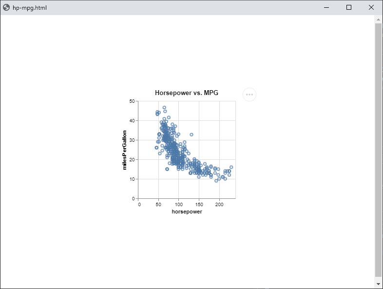
Your first plot
Data sources
The data property
tells Vega where the data for the plot is. Most, but not all,
specifications have a single, top level data property, e.g.
"data": {"url": "data/cars.json"}
Lisp-Stat allows you to use a data-frame, or data-frame
transformation (filter, selection, etc) as the value for the
data property. For example, since a data-frame transformation
returns a data-frame, we can insert the results as the data value,
as in this plot of residuals:
(:data (:values ,(filter-rows imdb
                              '(and (not (eql imdb-rating :na))
	                                (lt:timestamp< release-date
				                      (lt:parse-timestring "2019-01-01"))))
 :transform #((:joinaggregate #((:op :mean
	                             :field :imdb-rating
				                 :as :average-rating)))
where we remove :NA and any release-date after 2018.
Vega has
transformations
as well, but are a bit clumsy compared to those in Lisp-Stat.
Sometimes though, you’ll need them because a particular transformation
is not something you want to do to your data-frame. You can mix
transformations in a single plot, as we saw above in the residuals
plot, where the filtering was done in your data-frame and the
transformation was done in vega-lite.
Below are several examples of the hp-mpg plot, using various data sources:
Embedded
Most of the examples in this documentation use embedded data, where the data is a part of the plot specification. For completeness sake, we repeat an example here:
(plot:plot
  (vega:defplot hp-mpg
  `(:title "Vega Cars Horsepower vs. MPG"
    :description "Horsepower vs miles per gallon for various cars"
    :data (:values ,vgcars)
    :mark :point
	:encoding (:x (:field :horsepower :type :quantitative)
	           :y (:field :miles-per-gallon :type :quantitative)))))
URL
Note in this example we do not use a data frame as a source, therefore we have to specify field encodings as strings, since variable names will not have been converted to idiomatic lisp. E.g. Miles_per_Gallon vs miles-per-gallon.
(plot:plot
  (vega:defplot hp-mpg
    `(:title "Horsepower vs. MPG"
      :description "Horsepower vs miles per gallon for various cars"
      :data (:url "https://raw.githubusercontent.com/vega/vega-datasets/next/data/cars.json")
      :mark :point
      :encoding (:x (:field "Horsepower" :type :quantitative)
	             :y (:field "Miles_per_Gallon" :type :quantitative)))))
In a production environment, you may have several quri data sources in your image. To load from one of these:
(plot:plot
  (vega:defplot hp-mpg
    `(:title "Horsepower vs. MPG"
      :description "Horsepower vs miles per gallon for various cars"
      :data (:url ,(quri:uri "https://raw.githubusercontent.com/vega/vega-datasets/next/data/cars.json"))
      :mark :point
      :encoding (:x (:field "Horsepower" :type :quantitative)
	             :y (:field "Miles_per_Gallon" :type :quantitative)))))
Here we create the quri object at the same time, since it’s a stand-alone example. It would probably already be created in an actual use case.
Named data
Vega has named data sources that are useful if you have to refer to the same data in several places. We can create one like this:
(plot:plot
  (vega:defplot hp-mpg
    `(:title "Horsepower vs. MPG"
      :description "Horsepower vs miles per gallon for various cars"
      :datasets (:my-data ,vgcars)
      :data (:name :my-data)
      :mark :point
      :encoding (:x (:field :horsepower :type :quantitative)
	             :y (:field :miles-per-gallon :type :quantitative)))))
Plot specifications
Lisp in a spec
A plot specification is a plist. A nested plist to be exact
(or, perhaps more correctly, a tree). This means that we can use
Common Lisp tree/list functions to manipulate it.
If you look carefully at the examples, you’ll note they use a
backquote
(`) instead of a normal list quote ('). This is the mechanism
that Common Lisp
macros use to
rewrite code before compilation, and we can use the same mechanism to
rewrite our Vega-Lite specifications before encoding them.
The simplest, and most common, feature is insertion, like we did
above. By placing a comma (,) before the name of the data frame, we
told the backquote system to insert the value of the data frame
instead of the symbol (vgcars) in the example.
There’s a lot more you can do with the backquote mechanism. We won’t say any more here, as it’s mostly a topic for advanced users. It’s important for you to know it’s there though.
Properties
properties are the keys in key/value pairs. This is true whether
discussing a plist or JSON specification. Vega-Lite is case
sensitive and Common Lisp is not, so there are a few rules you need to
be aware of when constructing plot specifications.
Keys vs. values
Plot uses yason to transform a
plist plot specification to JSON. When yason encodes a spec
there are two functions of importance:
*symbol-encoder**symbol-key-encoder*
The former encodes values, and the latter encodes keys. In
PLOT, both of these are bound to a custom function
encode-symbol-as-metadata. This function does more than just encode
meta data though, it also handles naming conventions.
This won’t mean much in your day-to-day use of the system, but you do need to be aware of the difference between encoding a key and a value. There are some values that the encoder can’t work with, and in those cases you’ll need to use text.
Finally, remember that the symbol encoders are just a convenience to make things more lisp-like. You can build a plot specification, both keys and values, entirely from text if you wish.
Encoding symbols
JavaScript identifiers are incompatible with Common Lisp identifiers,
so we need a way to translate between them. plot uses Parenscript
symbol
conversion
for this. This is one of the reasons for specialised symbol encoders.
Let’s look at the difference between the standard yason encoder and
the one provided by plot (Parenscript):
LS-USER> (ps:symbol-to-js-string :x-offset)
"xOffset"
LS-USER> (yason:encode-symbol-as-lowercase :x-offset)
"x-offset"
LS-USER>
That difference is significant to Vega-Lite, where identifiers with a
- are not allowed. Vega is also case sensitive, so if a key is
xOffset, xoffset will not work. Fortunately Parenscript’s symbol
conversion is just what we need. It will automatically capitalise the
words following a dash, so x-offset becomes xOffset.
Symbols can also be used for value fields, and these are more forgiving. As long as you are consistent, and keep in mind that a behind the scenes conversion is happening, you can use lisp-like identifiers. Where this mostly comes into play is when you are using Vega transforms, as in the residuals example:
(:data ,(filter-rows imdb '(and (not (eql imdb-rating :na))
				                (lt:timestamp<
								      release-date
				                      (lt:parse-timestring "2019-01-01"))))
 :transform #((:joinaggregate #((:op :mean
	                             :field :imdb-rating
				                 :as :average-rating)))
             (:calculate "datum['imdbRating'] - datum.averageRating"
		      :as :rating-delta))
Notice that we used :imdb-rating as the field name for the
joinaggregate, however in the calculate part of the transform we
used the converted name imdbRating; that’s because by the time the
transform is run, the conversion will have already happened. When we
use :as we are assigning a name, when we use datum, we are
telling Vega to find a name, and since this is done in a text
field, plot won’t convert the names it finds inside text strings.
Finally, remember that the Parenscript transformation is also run on
variable/column names. You can see that we referred to imdb-rating
in the filter. If you get confused, run (keys <data-frame>) and
think about how ps:symbol-to-js-string would return the keys.
That’s what Vega will use as the column names.
This is more complicated to explain than to use. See the examples for best practice patterns. You’ll probably only need to be aware of this when doing transforms in Vega.
Variable symbols
When you define a data frame using the defdf macro, Lisp-Stat sets
up an environment for that data set. Part of that environment
includes configuring a package with a symbol for each variable in the
data set. These symbols have properties that describe the variable,
such as unit, label, type, etc. plot can make use of this
information when creating plots. Here’s a previous example, where we
do not use variable symbols:
(plot:plot
  (vega:defplot hp-mpg-plot
  `(:title "Vega Cars"
    :data (:values ,vgcars)
    :mark :point
	:encoding (:x (:field :horsepower :type :quantitative)
	           :y (:field :miles-per-gallon :type :quantitative)))))
and one where we do:
(plot:plot
  (vega:defplot hp-mpg-plot
  `(:title "Vega Cars"
    :data ,vgcars
    :mark :point
    :encoding (:x (:field vgcars:horsepower)
	           :y (:field vgcars:miles-per-gallon)))))
The difference is subtle, but this can save some typing if you are always adding titles and field types. We don’t use this in the examples because we want to demonstrate the lowest common denominator, but in all plots we create professionally we use variable symbols.
Special characters
There are occasions when neither the Parenscript encoder nor Yason
will correctly encode a key or value. In those situations, you’ll
need to use text strings. This can happen when Vega wants an encoding
that includes a character that is a reader macro, #, often used in
color specifications, or in format properties, like this one
(:format ".1~%")
Finally, there may be times when you need to use multiple escape
characters
instead of quoted strings. Occasionally an imported data set will
include parenthesis (). The data-frame reader will enclose these
in multiple escape characters, so for example a variable named body mass (g) will be loaded as |BODY-MASS-(G)|. In these cases you can
either change the name to a valid Common Lisp identifier using
rename-column!, or refer to the variable using the multiple escape
characters.
nil, null, false, true
Strictly speaking, false in JavaScript is the Boolean negative. In
practice, "false", a string, is often accepted. This seems to vary
within Vega-Lite. Some parts accept "false", others do not. The
plot symbol encoder will correctly output false for the symbol
:false, and you should use that anywhere you encounter a Boolean
negative.
true is encoded for the lisp symbol T.
nil and null may be entered directly as they are and will be
correctly transcribed.
Embedded data
By default, plot embeds data within the Vega-Lite JSON spec, then
uses vega-embed to display it
within an HTML page. The alternative is to use data from a
url. Both are
mostly equivalent, however there can be differences in parsing,
especially with dates. When data is embedded, values are parsed by
the JavaScript parser in your browser. When it’s loaded via a url,
it’s run through the Vega-Lite parser. Sometimes Vega-Lite needs a
bit of help by way
of format for
embedded data. For this reason plot always outputs dates & times in
ISO-8601 format, which works everywhere.
Large data sets can be problematic if you have a number of plots open and limited memory.
Saving plots
You can save plot specifications like any other Common Lisp object,
for example using with-open-file. data-frames also have read/write
functions. This section describes some convenience functions for plot
I/O.
Devices
A ‘device’ is a loose abstraction for the various locations that data
and specifications can be written to. For example in developing this
website, data is written to a directory for static files
/static/data/, and the plot specification to /static/plots/. We
can model this with a plist like so:
(defparameter hugo-url
  '(:spec-loc #P"s:/src/documentation/static/plots/"
	:data-loc #P"s:/src/documentation/static/data/"
	:data-url "/data/")
With this ‘device’, you can save a plot like so:
(vega:plot-to-device hugo-url <plot-name>)
and all the bits will be saved to their proper locations. See the
examples at the bottom of the file PLOT:SRC;VEGA;device.lisp for
various ways to use devices and the heuristics for determining
where/when/what to write. These devices have worked in practice in
generating more than 300 plots, but if you encounter a use case that’s
not covered, please open an
issue.
Vega quirks
Vega and Vega-Lite have more than their fair share of quirks and inconsistencies. For the most part you’ll only notice this in the ‘grammar’ of the graphics specification, however occasionally they may look like bugs.
When using the bin transformation, Vega-Lite assumes that if you
don’t provide the variable identifier to store the end of the bin, it
will use the name of the start of the bin, suffixed with _end. Many
of the Vega-Lite examples make this assumption. For example, this is
the snippet from a Vega-Lite example:
"data": {"url": "data/cars.json"},
  "transform": [{
      "bin": true, "field": "Horsepower", "as": "bin_Horsepwoer"
    }, {
      "aggregate": [{"op": "count", "as": "Count"}],
      "groupby": ["bin_Horsepwoer", "bin_Horsepwoer_end"]
    }, {
      "joinaggregate": [{"op": "sum", "field": "Count", "as": "TotalCount"}]
    }, {
      "calculate": "datum.Count/datum.TotalCount", "as": "PercentOfTotal"
    }
  ]
Noticed the bin is using as: bin_Horsepower and then later, in
the groupBy transformation, referring to bin_Horsepower_end. To
work around this ‘feature’, we need to specify both the start and end
for the bin operation:
:transform #((:bin t
              :field :horsepower
              :as #(:bin-horsepower :bin-horsepower-end))
                   (:aggregate #((:op :count :as :count))
                    :groupby #(:bin-horsepower :bin-horsepower-end))
This kind of behaviour may occur elsewhere, and it’s not well
documented, so just be careful when you see any kind of beginning or
end encoding in a Vega-Lite example.
Workflow
There are many possible workflows when plotting. This section describes a few that I’ve found useful when developing plots.
By default, plot will embed data in an HTML file and then call the
systems browser to open it. This is a perfectly fine way to develop plots,
especially if you’re on a machine with a good amount of RAM.
Vega-Desktop
The Vega-Desktop sadly now unmaintained, still works fine for Vega-Lite up to version 5. With this desktop application, you can drag a plot specification to the application and ‘watch’ it. Once watched, any changes you make are instantly updated in the application window. Here’s a demonstration:
First, set up a ‘device’ to use a directory on the desktop for plotting:
(defparameter vdsk1 '(:spec-loc #P"~/Desktop/plots/"
		              :data-loc #P"~/Desktop/plots/data/")
  "Put data into a data/ subdirectory")
Now send a scatterplot to this device:
(vega:plot-to-device vdsk1
  (vega:defplot hp-mpg
  `(:data (:values ,vgcars)
    :mark :point
	:encoding (:x (:field :horsepower :type :quantitative)
	           :y (:field :miles-per-gallon :type :quantitative)))))
Now drag the file ~/Desktop/plots/hp-mpg.vl.json to the Vega-Desktop
application:
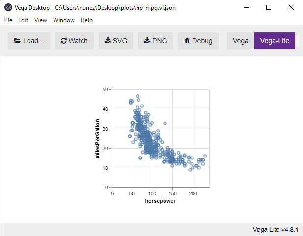
and click on the ‘watch’ button:
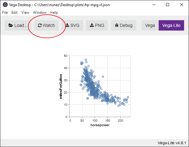
now go back to the buffer with the spec and add a title:
(vega:plot-to-device vdsk1
  (vega:defplot hp-mpg
  `(:title "Horsepower vs. Miles per Gallon"
    :data (:values ,vgcars)
    :mark :point
	:encoding (:x (:field :horsepower :type "quantitative")
	           :y (:field :miles-per-gallon :type "quantitative")))))
and reevaluate the form. If you’re in emacs, this is the C-x C-e
command. Observe how the plot is instantly updated:
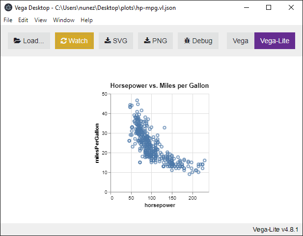
I tend to use this method when I’m tweaking a plot for final publication.
Vega edit
You can publish a plot specification to a Github gist and then invoke the Vega editor. This isn’t quite as real-time as Vega Desktop in that changes in the Lisp image aren’t automatically reflected and you’ll have to re-publish. It is a good way to debug plots and download them in various formats, or for sharing.
To use this mechanism, you’ll need to configure two environment variables so the gist wrapper will be able to use your credentials to authenticate to the Github API. Set the following environment variables to hold your github credentials:
- GITHUB_USERNAME
- GITHUB_OAUTH_TOKEN
Github no longer works with a password, so don’t bother setting that. If you want a custom scheme for authentication, you can create one by following the examples in examples/1.credentials.lisp
Now, you can edit the hp-mpg plot online with:
(vega:edit hp-mpg)
Debugging
There are a couple of commonly encountered scenarios when plots don’t display correctly:
- it’s so broken the browser displays nothing
- the
...button appears, but the plot is broken
Nothing is displayed
In this case, your best option is to print to a device where you can
examine the output. I use the Vega-Desktop (vgdsk1) so often it’s
part of my Lisp-Stat initialisation, and I also use it for these
cases. Once you’ve got the spec written out as JSON, see if
Vega-Desktop can render it, paying attention to the warnings.
Vega-Desktop also has a debug function:
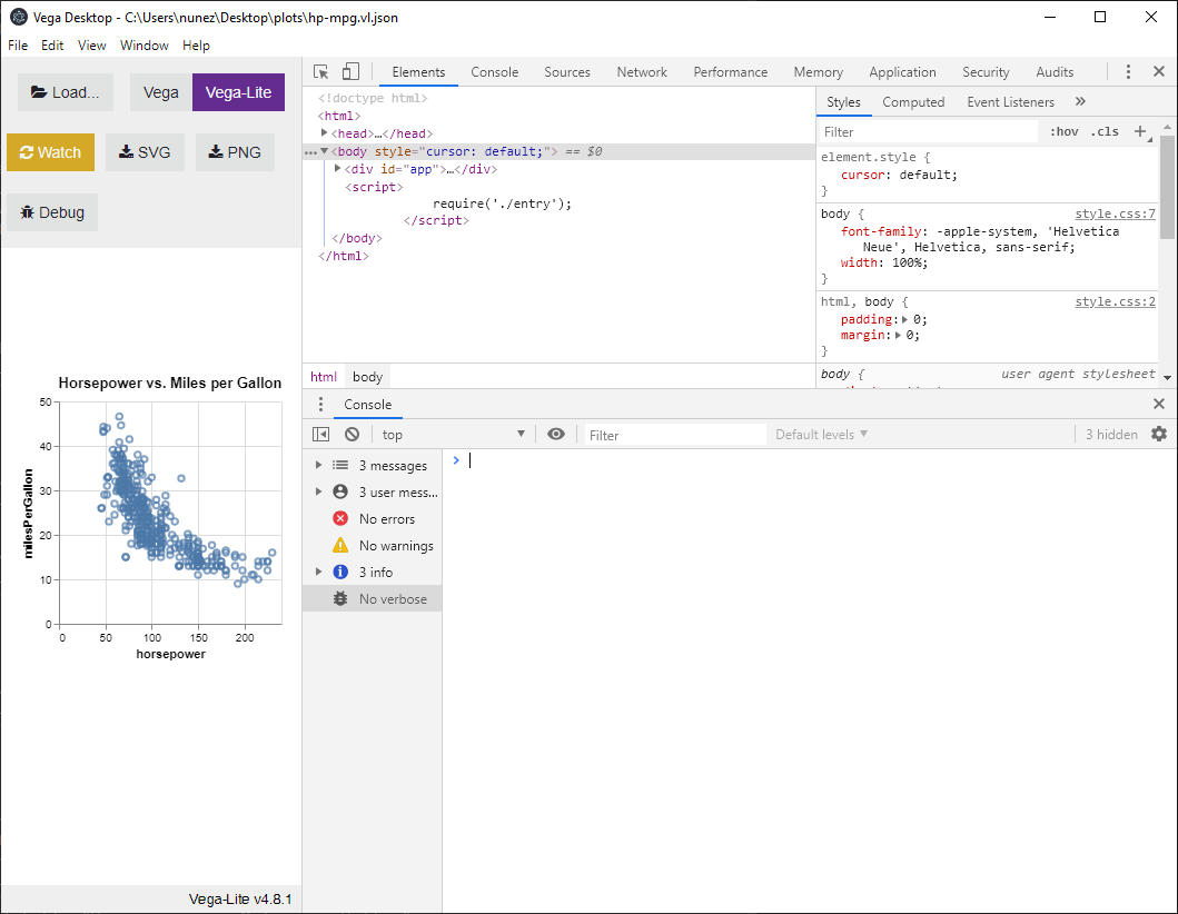
If Vega-Desktop doesn’t help, open the file in Visual Studio code, which has a schema validator. Generally these kinds of syntax errors are easy to spot once they’re pointed out by Visual Studio.
Something is displayed
If you see the three ellipses, then you can open the plot in the online vega editor. This is very similar to Vega Desktop, but with one important difference: you can only debug plots with embedded data sets or remotely available URLs. Because the online editor is a web application hosted on Github, you can’t access local data sets. This is one reason I typically use the Vega-Desktop / Visual Studio combination.
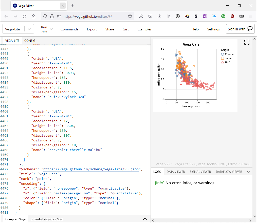
Getting plot information
There are two ways to get information about the plots in your environment.
show-plots
The show-plots command will display the plots you have defined,
along with a description (if one was provided in the spec). Here are
the plots currently in my environment:
LS-USER> (vega:show-plots)

0: #<PLOT GROUPED-BAR-CHART: Bar chart
NIL>

1: #<PLOT HP-MPG-PLOT: Scatter plot
NIL>

2: #<PLOT HP-MPG: Scatter plot
Horsepower vs miles per gallon for various cars>
Only the last, from the example above, has a description.
describe
You can also use the describe command to view plot information:
LS-USER> (describe hp-mpg)
HP-MPG
  Scatter plot of VGCARS
  Horsepower vs miles per gallon for various cars
inspect
By typing the plots name in the emacs REPL, a ‘handle’ of sorts is returned, printed in orange:
Right click on the orange text to get a context menu allowing various operations on the object, one of which is to ‘inspect’ the object.
Included datasets
The vega package includes all the data sets in the vega data
sets. They
have the same name, in the vega package, e.g. vega:penguins.