This section describes the core APIs and systems that comprise Lisp-Stat. These APIs include both the high level functionality described elsewhere, as well as lower level APIs that they are built on. This section will be of interest to ‘power users’ and developers who wish to extend Lisp-Stat, or build modules of their own.
This is the multi-page printable view of this section. Click here to print.
System Manuals
Manuals for Lisp-Stat systems
- 1: Array Operations
- 2: Data Frame
- 3: Distributions
- 4: Linear Algebra
- 5: Select
- 6: SQLDF
- 7: Statistics
1 - Array Operations
Manipulating sample data as arrays
Overview
The array-operations system contains a collection of functions and
macros for manipulating Common Lisp arrays and performing numerical
calculations with them.
Array-operations is a ‘generic’ way of operating on array like data
structures. Several aops functions have been implemented for
data-frame. For those that haven’t, you can transform arrays to
data frames using the df:matrix-df function, and a data-frame to an
array using df:as-array. This make it convenient to work with the
data sets using either system.
Quick look
Arrays can be created with numbers from a statistical distribution:
(rand '(2 2)) ; => #2A((0.62944734 0.2709539) (0.81158376 0.6700171))
in linear ranges:
(linspace 1 10 7) ; => #(1 5/2 4 11/2 7 17/2 10)
or generated using a function, optionally given index position
(generate #'identity '(2 3) :position) ; => #2A((0 1 2) (3 4 5))
They can also be transformed and manipulated:
(defparameter A #2A((1 2)
                    (3 4)))
(defparameter B #2A((2 3)
                    (4 5)))

;; split along any dimension
(split A 1)  ; => #(#(1 2) #(3 4))

;; stack along any dimension
(stack 1 A B) ; => #2A((1 2 2 3)
              ;        (3 4 4 5))

;; element-wise function map
(each #'+ #(0 1 2) #(2 3 5)) ; => #(2 4 7)

;; element-wise expressions
(vectorize (A B) (* A (sqrt B))) ; => #2A((1.4142135 3.4641016)
                                 ;        (6.0       8.944272))

;; index operations e.g. matrix-matrix multiply:
(each-index (i j)
  (sum-index k
    (* (aref A i k) (aref B k j)))) ; => #2A((10 13)
	                                ;        (22 29))
Array shorthand
The library defines the following short function names that are synonyms for Common Lisp operations:
| array-operations | Common Lisp |
|---|---|
| size | array-total-size |
| rank | array-rank |
| dim | array-dimension |
| dims | array-dimensions |
| nrow | number of rows in matrix |
| ncol | number of columns in matrix |
The array-operations package has the nickname aops, so you can use,
for example, (aops:size my-array) without use‘ing the package.
Displaced arrays
According to the Common Lisp specification, a displaced array is:
An array which has no storage of its own, but which is instead indirected to the storage of another array, called its target, at a specified offset, in such a way that any attempt to access the displaced array implicitly references the target array.
Displaced arrays are one of the niftiest features of Common Lisp. When an array is displaced to another array, it shares structure with (part of) that array. The two arrays do not need to have the same dimensions, in fact, the dimensions do not be related at all as long as the displaced array fits inside the original one. The row-major index of the former in the latter is called the offset of the displacement.
displace
Displaced arrays are usually constructed using make-array, but this
library also provides displace for that purpose:
(defparameter *a* #2A((1 2 3)
                      (4 5 6)))
(aops:displace *a* 2 1) ; => #(2 3)
Here’s an example of using displace to implement a sliding window over some set of values, say perhaps a time-series of stock prices:
(defparameter stocks (aops:linspace 1 100 100))
(loop for i from 0 to (- (length stocks) 20)
      do (format t "~A~%" (aops:displace stocks 20 i)))
;#(1 2 3 4 5 6 7 8 9 10 11 12 13 14 15 16 17 18 19 20)
;#(2 3 4 5 6 7 8 9 10 11 12 13 14 15 16 17 18 19 20 21)
;#(3 4 5 6 7 8 9 10 11 12 13 14 15 16 17 18 19 20 21 22)
flatten
flatten displaces to a row-major array:
(aops:flatten *a*) ; => #(1 2 3 4 5 6)
split
The real fun starts with split, which splits off sub-arrays nested
within a given axis:
(aops:split *a* 1) ; => #(#(1 2 3) #(4 5 6))
(defparameter *b* #3A(((0 1) (2 3))
                      ((4 5) (6 7))))
(aops:split *b* 0) ; => #3A(((0 1) (2 3)) ((4 5) (6 7)))
(aops:split *b* 1) ; => #(#2A((0 1) (2 3)) #2A((4 5) (6 7)))
(aops:split *b* 2) ; => #2A((#(0 1) #(2 3)) (#(4 5) #(6 7)))
(aops:split *b* 3) ; => #3A(((0 1) (2 3)) ((4 5) (6 7)))
Note how splitting at 0 and the rank of the array returns the array
itself.
sub
Now consider sub, which returns a specific array, composed of the
elements that would start with given subscripts:
(aops:sub *b* 0) ; => #2A((0 1)
                 ;        (2 3))
(aops:sub *b* 0 1) ; => #(2 3)
(aops:sub *b* 0 1 0) ; => 2
In the case of vectors, sub works like aref:
(aops:sub #(1 2 3 4 5) 1) ; => 2
There is also a (setf sub) function.
partition
partition returns a consecutive chunk of an array separated along its
first subscript:
(aops:partition #2A((0 1)
                    (2 3)
                    (4 5)
                    (6 7)
                    (8 9))
              1 3) ; => #2A((2 3)
			       ;        (4 5))
and also has a (setf partition) pair.
combine
combine is the opposite of split:
(aops:combine #(#(0 1) #(2 3))) ; => #2A((0 1)
                                ;        (2 3))
subvec
subvec returns a displaced subvector:
(aops:subvec #(0 1 2 3 4) 2 4) ; => #(2 3)
There is also a (setf subvec) function, which is like (setf subseq)
except for demanding matching lengths.
reshape
Finally, reshape can be used to displace arrays into a different
shape:
(aops:reshape #2A((1 2 3)
                  (4 5 6)) '(3 2))
; => #2A((1 2)
;        (3 4)
;        (5 6))
You can use t for one of the dimensions, to be filled in
automatically:
(aops:reshape *b* '(1 t)) ; => #2A((0 1 2 3 4 5 6 7))
reshape-col and reshape-row reshape your array into a column or row
matrix, respectively:
(defparameter *a* #2A((0 1)
                      (2 3)
					  (4 5)))
(aops:reshape-row *a*) ;=> #2A((0 1 2 3 4 5))
(aops:reshape-col *a*) ;=> #2A((0) (1) (2) (3) (4) (5))
Specifying dimensions
Functions in the library accept the following in place of dimensions:
- a list of dimensions (as for
make-array), - a positive integer, which is used as a single-element list,
- another array, the dimensions of which are used.
The last one allows you to specify dimensions with other arrays. For
example, to reshape an array a1 to look like a2, you can use
(aops:reshape a1 a2)
instead of the longer form
(aops:reshape a1 (aops:dims a2))
Creation & transformation
Use the functions in this section to create commonly used arrays
types. When the resulting element type cannot be inferred from an
existing array or vector, you can pass the element type as an optional
argument. The default is elements of type T.
Element traversal order of these functions is unspecified. The reason for this is that the library may use parallel code in the future, so it is unsafe to rely on a particular element traversal order.
The following functions all make a new array, taking the dimensions as
input. There are also versions ending in ! which do not make a
new array, but take an array as first argument, which is modified and
returned.
| Function | Description |
|---|---|
| zeros | Filled with zeros |
| ones | Filled with ones |
| rand | Filled with uniformly distributed random numbers between 0 and 1 |
| randn | Normally distributed with mean 0 and standard deviation 1 |
| linspace | Evenly spaced numbers in given range |
For example:
(aops:zeros 3)
; => #(0 0 0)

(aops:zeros 3 'double-float)
; => #(0.0d0 0.0d0 0.0d0)

(aops:rand '(2 2))
; => #2A((0.6686077 0.59425664)
;        (0.7987722 0.6930506))

(aops:rand '(2 2) 'single-float)
; => #2A((0.39332366 0.5557821)
;        (0.48831415 0.10924244))

(let ((a (make-array '(2 2) :element-type 'double-float)))
  ;; Modify array A, filling with random numbers
  ;; element type is taken from existing array
  (aops:rand! a))
  ; => #2A((0.6324615478515625d0 0.4636608362197876d0)
  ;        (0.4145939350128174d0 0.5124958753585815d0))
(linspace 0 4 5)   ;=> #(0 1 2 3 4)
(linspace 1 3 5)   ;=> #(0 1/2 1 3/2 2)
(linspace 1 3 5 'double-float) ;=> #(1.0d0 1.5d0 2.0d0 2.5d0 3.0d0)
(linspace 0 4d0 3) ;=> #(0.0d0 2.0d0 4.0d0)
generate
generate (and generate*) allow you to generate arrays using
functions. The function signatures are:
generate* (element-type function dimensions &optional arguments)
generate (function dimensions &optional arguments)
Where arguments are passed to function. Possible arguments are:
- no arguments, when ARGUMENTS is nil
- the position (= row major index), when ARGUMENTS is :POSITION
- a list of subscripts, when ARGUMENTS is :SUBSCRIPTS
- both when ARGUMENTS is :POSITION-AND-SUBSCRIPTS
(aops:generate (lambda () (random 10)) 3) ; => #(6 9 5)

(aops:generate #'identity '(2 3) :position) ; => #2A((0 1 2)
                                            ;        (3 4 5))

(aops:generate #'identity '(2 2) :subscripts)
; => #2A(((0 0) (0 1))
;        ((1 0) (1 1)))

(aops:generate #'cons '(2 2) :position-and-subscripts)
; => #2A(((0 0 0) (1 0 1))
;        ((2 1 0) (3 1 1)))
permute
permute can permute subscripts (you can also invert, complement, and
complete permutations, look at the docstring and the unit tests).
Transposing is a special case of permute:
(defparameter *a* #2A((1 2 3)
                      (4 5 6)))
(aops:permute '(0 1) *a*) ; => #2A((1 2 3)
                          ;        (4 5 6))
(aops:permute '(1 0) *a*) ; => #2A((1 4)
                          ;        (2 5)
						  ;        (3 6))
each
each applies a function to its one dimensional array arguments
elementwise. It essentially is an element-wise function map on each of
the vectors:
(aops:each #'+ #(0 1 2)
               #(2 3 5)
			   #(1 1 1)
; => #(3 5 8)
vectorize
vectorize is a macro which performs elementwise operations
(defparameter a #(1 2 3 4))
(aops:vectorize (a) (* 2 a)) ; => #(2 4 6 8)

(defparameter b #(2 3 4 5))
(aops:vectorize (a b) (* a (sin b)))
; => #(0.9092974 0.28224 -2.2704074 -3.8356972)
There is also a version vectorize* which takes a type argument for the
resulting array, and a version vectorize! which sets elements in a
given array.
margin
The semantics of margin are more difficult to explain, so perhaps an
example will be more useful. Suppose that you want to calculate column
sums in a matrix. You could permute (transpose) the matrix, split
its sub-arrays at rank one (so you get a vector for each row), and apply
the function that calculates the sum. margin automates that for you:
(aops:margin (lambda (column)
               (reduce #'+ column))
           #2A((0 1)
               (2 3)
               (5 7)) 0) ; => #(7 11)
But the function is more general than this: the arguments inner and
outer allow arbitrary permutations before splitting.
recycle
Finally, recycle allows you to reuse the elements of the first argument, object, to create new arrays by extending the dimensions. The :outer keyword repeats the original object and :inner keyword argument repeats the elements of object. When both :inner and :outer are nil, object is returned as is. Non-array objects are intepreted as rank 0 arrays, following the usual semantics.
(aops:recycle #(2 3) :inner 2 :outer 4)
; => #3A(((2 2) (3 3))
         ((2 2) (3 3))
         ((2 2) (3 3))
	     ((2 2) (3 3)))
Three dimensional arrays can be tough to get your head around. In the example above, :outer asks for 4 2-element vectors, composed of repeating the elements of object twice, i.e. repeat ‘2’ twice and repeat ‘3’ twice. Compare this with :inner as 3:
(aops:recycle #(2 3) :inner 3 :outer 4)
; #3A(((2 2 2) (3 3 3))
      ((2 2 2) (3 3 3))
	  ((2 2 2) (3 3 3))
	  ((2 2 2) (3 3 3)))
The most common use case for recycle is to ‘stretch’ a vector so that it can be an operand for an array of compatible dimensions. In Python, this would be known as ‘broadcasting’. See the Numpy broadcasting basics for other use cases.
For example, suppose we wish to multiply array a, a size 4x3 with vector b of size 3, as in the figure below:
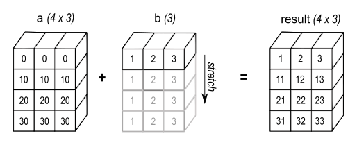
We can do that by recycling array b like this:
(recycle #(1 2 3) :outer 4)
;#2A((1 2 3)
;	 (1 2 3)
;	 (1 2 3)
;	 (1 2 3))
In a similar manner, the figure below (also from the Numpy page) shows how we might stretch a vector horizontally to create an array compatible with the one created above.
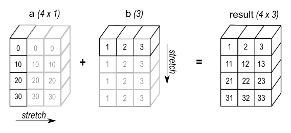
To create that array from a vector, use the :inner keyword:
(recycle #(0 10 20 30) :inner 3)
;#2A((0 0 0)
;	 (10 10 10)
;	 (20 20 20)
;	 (30 30 30))
turn
turn rotates an array by a specified number of clockwise 90° rotations. The axis of rotation is specified by RANK-1 (defaulting to 0) and RANK-2 (defaulting to 1). In the first example, we’ll rotate by 90°:
(defparameter array-1 #2A((1 0 0)
                          (2 0 0)
                          (3 0 0)))
(aops:turn array-1 1)
;; #2A((3 2 1)
;;     (0 0 0)
;;	   (0 0 0))
and if we rotate it twice (180°):
(aops:turn array-1 2)
;; #2A((0 0 3)
;;     (0 0 2)
;;     (0 0 1))
finally, rotate it three times (270°):
(aops:turn array-1 3)
;; #2A((0 0 0)
;;     (0 0 0)
;;     (1 2 3))
map-array
map-array maps a function over the elements of an array.
(aops:map-array #2A((1.7 2.1 4.3 5.4)
                    (0.3 0.4 0.5 0.6))
				#'log)
; #2A(( 0.53062826 0.7419373  1.4586151  1.686399)
;     (-1.2039728 -0.9162907 -0.6931472 -0.5108256))
outer
outer is generalized outer product of arrays using a provided function.
Lambda list: (function &rest arrays)
The resulting array has the concatenated dimensions of arrays
The examples below return the outer product of vectors or arrays. This is the outer product you get in most linear algebra packages.
(defparameter a #(2 3 5))
(defparameter b #(7 11))
(defparameter c #2A((7 11)
                    (13 17)))

(outer #'* a b)
;#2A((14 22)
;    (21 33)
;    (35 55))

(outer #'* c a)
;#3A(((14 21 35) (22 33 55))
;    ((26 39 65) (34 51 85)))
Indexing operations
nested-loop
nested-loop is a simple macro which iterates over a set of indices
with a given range
(defparameter A #2A((1 2) (3 4)))

(aops:nested-loop (i j) (array-dimensions A)
  (setf (aref A i j) (* 2 (aref A i j))))
A ; => #2A((2 4) (6 8))

(aops:nested-loop (i j) '(2 3)
  (format t "(~a ~a) " i j)) ; => (0 0) (0 1) (0 2) (1 0) (1 1) (1 2)
sum-index
sum-index is a macro which uses a code walker to determine the
dimension sizes, summing over the given index or indices
(defparameter A #2A((1 2) (3 4)))

;; Trace
(aops:sum-index i (aref A i i)) ; => 5

;; Sum array
(aops:sum-index (i j) (aref A i j)) ; => 10

;; Sum array
(aops:sum-index i (row-major-aref A i)) ; => 10
The main use for sum-index is in combination with each-index.
each-index
each-index is a macro which creates an array and iterates over the
elements. Like sum-index it is given one or more index symbols, and
uses a code walker to find array dimensions.
(defparameter A #2A((1 2)
                    (3 4)))
(defparameter B #2A((5 6)
                    (7 8)))

;; Transpose
(aops:each-index (i j) (aref A j i)) ; => #2A((1 3)
                                     ;        (2 4))

;; Sum columns
(aops:each-index i
  (aops:sum-index j
    (aref A j i))) ; => #(4 6)

;; Matrix-matrix multiply
(aops:each-index (i j)
   (aops:sum-index k
      (* (aref A i k) (aref B k j)))) ; => #2A((19 22)
	                                  ;        (43 50))
reduce-index
reduce-index is a more general version of sum-index; it
applies a reduction operation over one or more indices.
(defparameter A #2A((1 2)
                    (3 4)))

;; Sum all values in an array
(aops:reduce-index #'+ i (row-major-aref A i)) ; => 10

;; Maximum value in each row
(aops:each-index i
  (aops:reduce-index #'max j
    (aref A i j)))  ; => #(2 4)
Reducing
Some reductions over array elements can be done using the Common Lisp
reduce function, together with aops:flatten, which returns a
displaced vector:
(defparameter a #2A((1 2)
                    (3 4)))
(reduce #'max (aops:flatten a)) ; => 4
argmax & argmin
argmax and argmin find the row-major-aref index where an
array value is maximum or minimum. They both return two values: the
first value is the index; the second is the array value at that index.
(defparameter a #(1 2 5 4 2))
(aops:argmax a) ; => 2 5
(aops:argmin a) ; => 0 1
vectorize-reduce
More complicated reductions can be done with vectorize-reduce,
for example the maximum absolute difference between arrays:
(defparameter a #2A((1 2)
                    (3 4)))
(defparameter b #2A((2 2)
                    (1 3)))

(aops:vectorize-reduce #'max (a b) (abs (- a b))) ; => 2
best
best compares two arrays according to a function and returns the ‘best’ value found. The function, FN must accept two inputs and return true/false. This function is applied to elements of ARRAY. The row-major-aref index is returned.
Example: The index of the maximum is
   * (best #'> #(1 2 3 4))
    3   ; row-major index
    4   ; value
most
most finds the element of ARRAY that returns the value closest to positive infinity when FN is applied to the array value. Returns the row-major-aref index, and the winning value.
Example: The maximum of an array is:
     (most #'identity #(1 2 3))
     -> 2    (row-major index)
        3    (value)
and the minimum of an array is:
      (most #'- #(1 2 3))
        0
        -1
See also reduce-index above.
Scalar values
Library functions treat non-array objects as if they were equivalent to
0-dimensional arrays: for example, (aops:split array (rank array))
returns an array that effectively equivalent (eq) to array. Another
example is recycle:
(aops:recycle 4 :inner '(2 2)) ; => #2A((4 4)
                               ;        (4 4))
Stacking
You can stack compatible arrays by column or row. Metaphorically you can think of these operations as stacking blocks. For example stacking two row vectors yields a 2x2 array:
(stack-rows #(1 2) #(3 4))
;; #2A((1 2)
;;     (3 4))
Like other functions, there are two versions: generalised stacking,
with rows and columns of type T and specialised versions where the
element-type is specified. The versions allowing you to specialise
the element type end in *.
The stack functions use object dimensions (as returned by dims to
determine how to use the object.
- when the object has 0 dimensions, fill a column with the element
- when the object has 1 dimension, use it as a column
- when the object has 2 dimensions, use it as a matrix
copy-row-major-block is a utility function in the stacking package
that does what it suggests; it copies elements from one array to
another. This function should be used to implement copying of
contiguous row-major blocks of elements.
rows
stack-rows-copy is the method used to implement the copying of objects in stack-row*, by copying the elements of source to destination, starting with the row index start-row in the latter. Elements are coerced to element-type.
stack-rows and stack-rows* stack objects row-wise into an array of the given element-type, coercing if necessary. Always return a simple array of rank 2. stack-rows always returns an array with elements of type T, stack-rows* coerces elements to the specified type.
columns
stack-cols-copy is a method used to implement the copying of objects in stack-col*, by copying the elements of source to destination, starting with the column index start-col in the latter. Elements are coerced to element-type.
stack-cols and stack-cols* stack objects column-wise into an array of the given element-type, coercing if necessary. Always return a simple array of rank 2. stack-cols always returns an array with elements of type T, stack-cols* coerces elements to the specified type.
arbitrary
stack and stack* stack array arguments along axis. element-type determines the element-type
of the result.
(defparameter *a1* #(0 1 2))
(defparameter *a2* #(3 5 7))
(aops:stack 0 *a1* *a2*) ; => #(0 1 2 3 5 7)
(aops:stack 1
          (aops:reshape-col *a1*)
          (aops:reshape-col *a2*)) ; => #2A((0 3)
	                               ;        (1 5)
								   ;        (2 7))
2 - Data Frame
Manipulating data using a data frame
Overview
A common lisp data frame is a collection of observations of sample variables that shares many of the properties of arrays and lists. By design it can be manipulated using the same mechanisms used to manipulate lisp arrays. This allow you to, for example, transform a data frame into an array and use array-operations to manipulate it, and then turn it into a data frame again to use in modeling or plotting.
Data frame is implemented as a two-dimensional common lisp data structure: a vector of vectors for data, and a hash table mapping variable names to column vectors. All columns are of equal length. This structure provides the flexibility required for column oriented manipulation, as well as speed for large data sets.
Note
In this document we refer to column and variable interchangeably. Likewise factor and category refer to a variable type. Where necessary we distinguish the terminology.Load/install
Data-frame is part of the Lisp-Stat package. It can be used independently if desired. Since the examples in this manual use Lisp-Stat functionality, we’ll use it from there rather than load independently.
(ql:quickload :lisp-stat)
Within the Lisp-Stat system, the LS-USER package is the package for
you to do statistics work. Type the following to change to that
package:
(in-package :ls-user)
Note
The examples assume that you are in package LS-USER. You should make a habit of always working from theLS-USER
package. All the samples may be copied to the clipboard using the
copy button in the upper-right corner of the sample code
box.
Naming conventions
Lisp-Stat has a few naming conventions you should be aware of. If you see a punctuation mark or the letter ‘p’ as the last letter of a function name, it indicates something about the function:
- ‘!’ indicates that the function is destructive. It will modify the data that you pass to it. Otherwise, it will return a copy that you will need to save in a variable.
- ‘p’, ‘-p’ or ‘?’ means the function is a predicate, that is returns a Boolean truth value.
Data frame environment
Although you can work with data frames bound to symbols (as would
happen if you used (defparameter ...), it is more convenient to
define them as part of an environment. When you do this, the system
defines a package of the same name as the data frame, and provides a
symbol for each variable. Let’s see how things work without an
environment:
First, we define a data frame as a parameter:
(defparameter mtcars (read-csv rdata:mtcars)
"Motor Trend Car Road Tests")
;; WARNING: Missing column name was filled in
;; MTCARS2
Now if we want a column, we can say:
(column mtcars 'mpg)
Now let’s define an environment using defdf:
(defdf mtcars (read-csv rdata:mtcars)
"Motor Trend Car Road Tests")
;; WARNING: Missing column name was filled in
;; #<DATA-FRAME (32 observations of 12 variables)
;; Motor Trend Car Road Tests>
Now we can access the same variable with:
mtcars:mpg
defdf does a lot more than this, and you should probably use defdf to set up an environment instead of defparameter. We mention it here because there’s an important bit about maintaining the environment to be aware of:
Note
Destructive functions (those ending in ‘!’), will automatically update the environment for you. Functions that return a copy of the data will not.defdf
The defdf macro is conceptually equivalent to the Common
Lisp defparameter, but with some additional functionality that makes
working with data frames easier. You use it the same way you’d use
defparameter, for example:
(defdf foo <any-function returning a data frame> )
We’ll use both ways of defining data frames in this manual. The access
methods that are defined by defdf are described in the
access data section.
Data types
It is important to note that there are two ’types’ in Lisp-Stat: the
implementation type and the ‘statistical’ type. Sometimes these are
the same, such as in the case of reals; in other situations they are
not. A good example of this can be seen in the mtcars data set. The
hp (horsepower), gear and carb are all of type integer from an
implementation perspective. However only horsepower is a continuous
variable. You can have an additional 0.5 horsepower, but you cannot
add an additional 0.5 gears or carburetors.
Data types are one kind of property that can be set on a variable.
As part of the recoding and data cleansing process, you will want to add
properties to your variables. In Common Lisp, these are plists that
reside on the variable symbols, e.g. mtcars:mpg. In R they are
known as attributes. By default, there are three properties for
each variable: type, unit and label (documentation). When you load
from external formats, like CSV, these properties are all nil; when
you load from a lisp file, they will have been saved along with the
data (if you set them).
There are seven data types in Lisp-Stat:
- string
- integer
- double-float
- single-float
- categorical (
factorin R) - temporal
- bit (Boolean)
Numeric
Numeric types, double-float, single-float and integer are all
essentially similar. The vector versions have type definitions (from
the numeric-utilities package) of:
- simple-double-float-vector
- simple-single-float-vector
- simple-fixnum-vector
As an example, let’s look at mtcars:mpg, where we have a variable of
type float, but a few integer values mixed in.
The values may be equivalent, but the types are not. The CSV
loader has no way of knowing, so loads the column as a mixture of
integers and floats. Let’s start by reloading mtcars from the CSV
file:
(undef 'mtcars)
(defdf mtcars (read-csv rdata:mtcars))
and look at the mpg variable:
LS-USER> mtcars:mpg
#(21 21 22.8d0 21.4d0 18.7d0 18.1d0 14.3d0 24.4d0 22.8d0 19.2d0 17.8d0 16.4d0
  17.3d0 15.2d0 10.4d0 10.4d0 14.7d0 32.4d0 30.4d0 33.9d0 21.5d0 15.5d0 15.2d0
  13.3d0 19.2d0 27.3d0 26 30.4d0 15.8d0 19.7d0 15 21.4d0)
LS-USER> (type-of *)
(SIMPLE-VECTOR 32)
Notice that the first two entries in the vector are integers, and the
remainder floats. To fix this manually, you will need to coerce each
element of the column to type double-float (you could use
single-float in this case; as a matter of habit we usually use
double-float) and then change the type of the vector to a
specialised float vector.
You can use the heuristicate-types function to guess the statistical
types for you. For reals and strings, heuristicate-types works
fine, however because integers and bits can be used to encode
categorical or numeric values, you will have to indicate the type
using set-properties. We see this below with gear and carb,
although implemented as integer, they are actually type
categorical. The next sections describes how to set them.
Using describe, we can view the
types of all the variables that heuristicate-types set:
LS-USER> (heuristicate-types mtcars)
LS-USER> (describe mtcars)
MTCARS
  A data-frame with 32 observations of 12 variables

Variable | Type         | Unit | Label
-------- | ----         | ---- | -----------
X8       | STRING       | NIL  | NIL
MPG      | DOUBLE-FLOAT | NIL  | NIL
CYL      | INTEGER      | NIL  | NIL
DISP     | DOUBLE-FLOAT | NIL  | NIL
HP       | INTEGER      | NIL  | NIL
DRAT     | DOUBLE-FLOAT | NIL  | NIL
WT       | DOUBLE-FLOAT | NIL  | NIL
QSEC     | DOUBLE-FLOAT | NIL  | NIL
VS       | BIT          | NIL  | NIL
AM       | BIT          | NIL  | NIL
GEAR     | INTEGER      | NIL  | NIL
CARB     | INTEGER      | NIL  | NIL
Notice the system correctly typed vs and am as Boolean (bit)
(correct in a mathematical sense)
Strings
Unlike in R, strings are not considered categorical variables by default. Ordering of strings varies according to locale, so it’s not a good idea to rely on the strings. Nevertheless, they do work well if you are working in a single locale.
Categorical
Categorical variables have a fixed and known set of possible values.
In mtcars, gear, carb vs and am are categorical variables,
but heuristicate-types can’t distinguish categorical types, so
we’ll set them:
(set-properties mtcars :type '(:vs :categorical
			                    :am :categorical
			                    :gear :categorical
			                    :carb :categorical))
Temporal
Dates and times can be surprisingly complicated. To make working with
them simpler, Lisp-Stat uses vectors of
localtime objects to
represent dates & times. You can set a temporal type with
set-properties as well using the keyword :temporal.
Units & labels
To add units or labels to the data frame, use the set-properties
function. This function takes a plist of variable/value pairs, so to
set the units and labels:
(set-properties mtcars :unit '(:mpg m/g
	                   :cyl :NA
			           :disp in³
			           :hp hp
			           :drat :NA
			           :wt lb
			           :qsec s
			           :vs :NA
			           :am :NA
			           :gear :NA
			           :carb :NA))

(set-properties mtcars :label '(:mpg "Miles/(US) gallon"
				       :cyl "Number of cylinders"
                       :disp "Displacement (cu.in.)"
				       :hp "Gross horsepower"
				       :drat "Rear axle ratio"
				       :wt "Weight (1000 lbs)"
				       :qsec "1/4 mile time"
				       :vs "Engine (0=v-shaped, 1=straight)"
				       :am "Transmission (0=automatic, 1=manual)"
				       :gear "Number of forward gears"
				       :carb "Number of carburetors"))
Now look at the description again:
LS-USER> (describe mtcars)
MTCARS
  A data-frame with 32 observations of 12 variables

Variable | Type         | Unit | Label
-------- | ----         | ---- | -----------
X8       | STRING       | NIL  | NIL
MPG      | DOUBLE-FLOAT | M/G  | Miles/(US) gallon
CYL      | INTEGER      | NA   | Number of cylinders
DISP     | DOUBLE-FLOAT | IN3  | Displacement (cu.in.)
HP       | INTEGER      | HP   | Gross horsepower
DRAT     | DOUBLE-FLOAT | NA   | Rear axle ratio
WT       | DOUBLE-FLOAT | LB   | Weight (1000 lbs)
QSEC     | DOUBLE-FLOAT | S    | 1/4 mile time
VS       | BIT          | NA   | Engine (0=v-shaped, 1=straight)
AM       | BIT          | NA   | Transmission (0=automatic, 1=manual)
GEAR     | INTEGER      | NA   | Number of forward gears
CARB     | INTEGER      | NA   | Number of carburetors
You can set your own properties with this command too. To make your
custom properties appear in the describe command and be saved
automatically, override the describe and write-df methods, or use
:after methods.
Create data-frames
A data frame can be created from a Common Lisp array, alist,
plist, individual data vectors, another data frame or a vector-of
vectors. In this section we’ll describe creating a data frame from each of these.
Data frame columns represent sample set variables, and its rows are observations (or cases).
Note
For these examples we are going to install a modified version of the Lisp-Stat data-frame print-object function. This will cause the REPL to display the data-frame at creation, and save us from having to type (print-data data-frame) in each example. If you’d like to install it as we have, execute the code below at the REPL.(defmethod print-object ((df data-frame) stream)
"Print the first six rows of DATA-FRAME"
(let ((*print-lines* 6))
(df:print-data df stream nil)))
(set-pprint-dispatch 'df:data-frame
#'(lambda (s df) (df:print-data df s nil)))
You can ignore the warning that you’ll receive after executing the code above.
Let’s create a simple data frame. First we’ll setup some variables (columns) to represent our sample domain:
(defparameter v #(1 2 3 4)) ; vector
(defparameter b #*0110)     ; bits
(defparameter s #(a b c d)) ; symbols
(defparameter plist `(:vector ,v :symbols ,s)) ;only v & s
Let’s print plist. Just type the name in at the REPL prompt.
plist
(:VECTOR #(1 2 3 4) :SYMBOLS #(A B C D))
From p/a-lists
Now suppose we want to create a data frame from a plist
(apply #'df plist)

;; VECTOR SYMBOLS
;;      1       A
;;      2       B
;;      3       C
;;      4       D
We could also have used the plist-df function:
(plist-df plist)

;; VECTOR SYMBOLS
;;      1       A
;;      2       B
;;      3       C
;;      4       D
and to demonstrate the same thing using an alist, we’ll use the
alexandria:plist-alist function to convert the plist into an
alist:
(alist-df (plist-alist plist))

;; VECTOR SYMBOLS
;;      1       A
;;      2       B
;;      3       C
;;      4       D
From vectors
You can use make-df to create a data frame from keys and a list of
vectors. Each vector becomes a column in the data-frame.
(make-df '(:a :b)                 ; the keys
         '(#(1 2 3) #(10 20 30))) ; the columns
;; A  B
;; 1 10
;; 2 20
;; 3 30
This is useful if you’ve started working with variables defined with
defparameter or defvar and want to combine them into a data frame.
From arrays
matrix-df converts a matrix (array) to a data-frame with the given
keys.
(matrix-df #(:a :b) #2A((1 2)
	                    (3 4)))
;#<DATA-FRAME (2 observations of 2 variables)>
This is useful if you need to do a lot of numeric number-crunching on
a data set as an array, perhaps with BLAS or array-operations then
want to add categorical variables and continue processing as a
data-frame.
Example datasets
Vincent Arel-Bundock maintains a library of over 1700 R
datasets that is a
consolidation of example data from various R packages. You can load
one of these by specifying the url to the raw data to the read-csv
function. For example to load the
iris
data set, use:
(defdf iris
	(read-csv "https://raw.githubusercontent.com/vincentarelbundock/Rdatasets/master/csv/datasets/iris.csv")
	"Edgar Anderson's Iris Data")
Default datasets
To make the examples and tutorials easier, Lisp-Stat includes the URLs
for the R built in data sets. You can see these by viewing the
rdata:*r-default-datasets* variable:
LS-USER? rdata:*r-default-datasets*
(RDATA:AIRPASSENGERS RDATA:ABILITY.COV RDATA:AIRMILES RDATA:AIRQUALITY
 RDATA:ANSCOMBE RDATA:ATTENU RDATA:ATTITUDE RDATA:AUSTRES RDATA:BJSALES
 RDATA:BOD RDATA:CARS RDATA:CHICKWEIGHT RDATA:CHICKWTS RDATA:CO2-1 RDATA:CO2-2
 RDATA:CRIMTAB RDATA:DISCOVERIES RDATA:DNASE RDATA:ESOPH RDATA:EURO
 RDATA:EUSTOCKMARKETS RDATA:FAITHFUL RDATA:FORMALDEHYDE RDATA:FREENY
 RDATA:HAIREYECOLOR RDATA:HARMAN23.COR RDATA:HARMAN74.COR RDATA:INDOMETH
 RDATA:INFERT RDATA:INSECTSPRAYS RDATA:IRIS RDATA:IRIS3 RDATA:ISLANDS
 RDATA:JOHNSONJOHNSON RDATA:LAKEHURON RDATA:LH RDATA:LIFECYCLESAVINGS
 RDATA:LOBLOLLY RDATA:LONGLEY RDATA:LYNX RDATA:MORLEY RDATA:MTCARS RDATA:NHTEMP
 RDATA:NILE RDATA:NOTTEM RDATA:NPK RDATA:OCCUPATIONALSTATUS RDATA:ORANGE
 RDATA:ORCHARDSPRAYS RDATA:PLANTGROWTH RDATA:PRECIP RDATA:PRESIDENTS
 RDATA:PRESSURE RDATA:PUROMYCIN RDATA:QUAKES RDATA:RANDU RDATA:RIVERS
 RDATA:ROCK RDATA:SEATBELTS RDATA::STUDENT-SLEEP RDATA:STACKLOSS
 RDATA:SUNSPOT.MONTH RDATA:SUNSPOT.YEAR RDATA:SUNSPOTS RDATA:SWISS RDATA:THEOPH
 RDATA:TITANIC RDATA:TOOTHGROWTH RDATA:TREERING RDATA:TREES RDATA:UCBADMISSIONS
 RDATA:UKDRIVERDEATHS RDATA:UKGAS RDATA:USACCDEATHS RDATA:USARRESTS
 RDATA:USJUDGERATINGS RDATA:USPERSONALEXPENDITURE RDATA:USPOP RDATA:VADEATHS
 RDATA:VOLCANO RDATA:WARPBREAKS RDATA:WOMEN RDATA:WORLDPHONES RDATA:WWWUSAGE)
To load one of these, you can use the name of the data set. For example to load mtcars:
(defdf mtcars
  (read-csv rdata:mtcars))
If you want to load all of the default R data sets, use the
rdata:load-r-default-datasets command. All the data sets included in
base R will now be loaded into your environment. This is useful if you
are following a R tutorial, but using Lisp-Stat for the analysis
software.
You may also want to save the default R data sets in order to augment
the data with labels, units, types, etc. To save all of the default R
data sets to the LS:DATA;R directory, use the
(rdata:save-r-default-datasets) command if the default data sets
have already been loaded, or save-r-data if they have not. This
saves the data in lisp format.
Install R datasets
To work with all of the R data sets, we recommend you use git to
download the repository to your hard drive. For example I downloaded the
example data to the s: drive like this:
cd s:
git clone https://github.com/vincentarelbundock/Rdatasets.git
and setup a logical host in my ls-init.lisp file like so:
;;; Define logical hosts for external data sets
(setf (logical-pathname-translations "RDATA")
	`(("**;*.*.*" ,(merge-pathnames "csv/**/*.*" "s:/Rdatasets/"))))
Now you can access any of the datasets using the logical
pathname. Here’s an example of creating a data frame using the
ggplot mpg data set:
(defdf mpg (read-csv #P"RDATA:ggplot2;mpg.csv"))
Searching the examples
With so many data sets, it’s helpful to load the index into a data
frame so you can search for specific examples. You can do this by
loading the rdata:index into a data frame:
(defdf rindex (read-csv rdata:index))
I find it easiest to use the SQL-DF system to query this data. For example if you wanted to find the data sets with the largest number of observations:
(ql:quickload :sqldf)
(print-data
	(sqldf:sqldf "select item, title, rows, cols from rindex order by rows desc limit 10"))

;;   ITEM            TITLE                                                               ROWS COLS
;; 0 military        US Military Demographics                                         1414593    6
;; 1 Birthdays       US Births in 1969 - 1988                                          372864    7
;; 2 wvs_justifbribe Attitudes about the Justifiability of Bribe-Taking in the ...     348532    6
;; 3 flights         Flights data                                                      336776   19
;; 4 wvs_immig       Attitudes about Immigration in the World Values Survey            310388    6
;; 5 Fertility       Fertility and Women's Labor Supply                                254654    8
;; 6 avandia         Cardiovascular problems for two types of Diabetes medicines       227571    2
;; 7 AthleteGrad     Athletic Participation, Race, and Graduation                      214555    3
;; 8 mortgages       Data from "How do Mortgage Subsidies Affect Home Ownership? ..."  214144    6
;; 9 mammogram       Experiment with Mammogram Randomized
Export data frames
These next few functions are the reverse of the ones above used to create them. These are useful when you want to use foreign libraries or common lisp functions to process the data.
For this section of the manual, we are going to work with a subset of
the mtcars data set from above. We’ll use the
select package to take the first 5 rows so that
the data transformations are easier to see.
(defparameter mtcars-small (select mtcars (range 0 5) t))
The next three functions convert a data-frame to and from standard
common lisp data structures. This is useful if you’ve got data in
Common Lisp format and want to work with it in a data frame, or if
you’ve got a data frame and want to apply Common Lisp operators on it
that don’t exist in df.
as-alist
Just like it says on the tin, as-alist takes a data frame and
returns an alist version of it (formatted here for clearer output –
a pretty printer that outputs an alist in this format would be a
welcome addition to Lisp-Stat)
(as-alist mtcars-small)
;; ((MTCARS:X1 . #("Mazda RX4" "Mazda RX4 Wag" "Datsun 710" "Hornet 4 Drive" "Hornet Sportabout"))
;;  (MTCARS:MPG . #(21 21 22.8d0 21.4d0 18.7d0))
;;  (MTCARS:CYL . #(6 6 4 6 8))
;;  (MTCARS:DISP . #(160 160 108 258 360))
;;  (MTCARS:HP . #(110 110 93 110 175))
;;  (MTCARS:DRAT . #(3.9d0 3.9d0 3.85d0 3.08d0 3.15d0))
;;  (MTCARS:WT . #(2.62d0 2.875d0 2.32d0 3.215d0 3.44d0))
;;  (MTCARS:QSEC . #(16.46d0 17.02d0 18.61d0 19.44d0 17.02d0))
;;  (MTCARS:VS . #*00110)
;;  (MTCARS:AM . #*11100)
;;  (MTCARS:GEAR . #(4 4 4 3 3))
;;  (MTCARS:CARB . #(4 4 1 1 2)))
as-plist
Similarly, as-plist will return a plist:
(as-plist mtcars-small)
;; (MTCARS:X1 #("Mazda RX4" "Mazda RX4 Wag" "Datsun 710" "Hornet 4 Drive" "Hornet Sportabout")
;;  MTCARS:MPG #(21 21 22.8d0 21.4d0 18.7d0)
;;	MTCARS:CYL #(6 6 4 6 8)
;;	MTCARS:DISP #(160 160 108 258 360)
;;	MTCARS:HP #(110 110 93 110 175)
;;	MTCARS:DRAT #(3.9d0 3.9d0 3.85d0 3.08d0 3.15d0)
;;	MTCARS:WT #(2.62d0 2.875d0 2.32d0 3.215d0 3.44d0)
;;	MTCARS:QSEC #(16.46d0 17.02d0 18.61d0 19.44d0 17.02d0)
;;	MTCARS:VS #*00110
;;	MTCARS:AM #*11100
;;	MTCARS:GEAR #(4 4 4 3 3)
;;	MTCARS:CARB #(4 4 1 1 2))
as-array
as-array returns the data frame as a row-major two dimensional lisp
array. You’ll want to save the variable names using the
keys function to make it easy to
convert back (see matrix-df). One of the reasons you
might want to use this function is to manipulate the data-frame using
array-operations. This is
particularly useful when you have data frames of all numeric values.
(defparameter mtcars-keys (keys mtcars)) ; we'll use later
(defparameter mtcars-small-array (as-array mtcars-small))
mtcars-small-array
;; 0 Mazda RX4         21.0 6 160 110 3.90 2.620 16.46 0 1 4 4
;; 1 Mazda RX4 Wag     21.0 6 160 110 3.90 2.875 17.02 0 1 4 4
;; 2 Datsun 710        22.8 4 108  93 3.85 2.320 18.61 1 1 4 1
;; 3 Hornet 4 Drive    21.4 6 258 110 3.08 3.215 19.44 1 0 3 1
;; 4 Hornet Sportabout 18.7 8 360 175 3.15 3.440 17.02 0 0 3 2
Our abbreviated mtcars data frame is now a two dimensional Common
Lisp array. It may not look like one because Lisp-Stat will ‘print
pretty’ arrays. You can inspect it with the describe command to make
sure:
LS-USER> (describe mtcars-small-array)
...

Type: (SIMPLE-ARRAY T (5 12))
Class: #<BUILT-IN-CLASS SIMPLE-ARRAY>
Element type: T
Rank: 2
Physical size: 60
vectors
The columns function returns the variables of the data frame as a vector of
vectors:
(columns mtcars-small)
; #(#("Mazda RX4" "Mazda RX4 Wag" "Datsun 710" "Hornet 4 Drive" "Hornet Sportabout")
;   #(21 21 22.8d0 21.4d0 18.7d0)
;	#(6 6 4 6 8)
;	#(160 160 108 258 360)
;	#(110 110 93 110 175)
;	#(3.9d0 3.9d0 3.85d0 3.08d0 3.15d0)
;	#(2.62d0 2.875d0 2.32d0 3.215d0 3.44d0)
;	#(16.46d0 17.02d0 18.61d0 19.44d0 17.02d0)
;	#*00110
;	#*11100
;	#(4 4 4 3 3)
;	#(4 4 1 1 2))
This is a column-major lisp array.
You can also pass a selection to the columns function to return
specific columns:
(columns mtcars-small 'mpg)
; #(21 21 22.8d0 21.4d0 18.7d0)
The functions in array-operations are
helpful in further dealing with data frames as vectors and arrays. For
example you could convert a data frame to a transposed array by using
aops:combine with the
columns function:
(combine (columns mtcars-small))
;;  0 Mazda RX4 Mazda RX4 Wag Datsun 710 Hornet 4 Drive Hornet Sportabout
;;  1     21.00        21.000      22.80         21.400             18.70
;;  2      6.00         6.000       4.00          6.000              8.00
;;  3    160.00       160.000     108.00        258.000            360.00
;;  4    110.00       110.000      93.00        110.000            175.00
;;  5      3.90         3.900       3.85          3.080              3.15
;;  6      2.62         2.875       2.32          3.215              3.44
;;  7     16.46        17.020      18.61         19.440             17.02
;;  8      0.00         0.000       1.00          1.000              0.00
;;  9      1.00         1.000       1.00          0.000              0.00
;; 10      4.00         4.000       4.00          3.000              3.00
;; 11      4.00         4.000       1.00          1.000              2.00
Load data
There are two functions for loading data. The first data makes
loading from logical pathnames convenient. The other, read-csv
works with the file system or URLs. Although the name read-csv
implies only CSV (comma separated values), it can actually read with
other delimiters, such as the tab character. See the DFIO API
reference for more information.
The data command
For built in Lisp-Stat data sets, you can load with just the data set
name. For example to load mtcars:
(data :mtcars)
If you’ve installed the R data
sets, and want to load
the antigua data set from the daag package, you could do it like
this:
(data :antigua :system :rdata :directory :daag :type :csv)
If the file type is not lisp (say it’s TSV or CSV), you need to
specify the type parameter.
From strings
Here is a short demonstration of reading from strings:
(defparameter *d*
  (read-csv
   (format nil "Gender,Age,Height~@
              \"Male\",30,180.~@
              \"Male\",31,182.7~@
               \"Female\",32,1.65e2")))
dfio tries to hard to decipher the various number formats sometimes
encountered in CSV files:
(select (dfio:read-csv
                 (format nil "\"All kinds of wacky number formats\"~%.7~%19.~%.7f2"))
                t 'all-kinds-of-wacky-number-formats)
; => #(0.7d0 19.0d0 70.0)
From delimited files
We saw above that dfio can read from strings, so one easy way to
read from a file is to use the uiop system function
read-file-string. We can read one of the example data files
included with Lisp-Stat like this:
(read-csv
	(uiop:read-file-string #P"LS:DATA;absorbtion.csv"))
;;    IRON ALUMINUM ABSORPTION
;;  0   61       13          4
;;  1  175       21         18
;;  2  111       24         14
;;  3  124       23         18
;;  4  130       64         26
;;  5  173       38         26 ..
That example just illustrates reading from a file to a string. In practice you’re better off just reading the file in directly and avoid reading into a string first:
(read-csv #P"LS:DATA;absorbtion.csv")
;;    IRON ALUMINUM ABSORPTION
;;  0   61       13          4
;;  1  175       21         18
;;  2  111       24         14
;;  3  124       23         18
;;  4  130       64         26
;;  5  173       38         26 ..
From parquet files
You can use the duckdb system to load data from parquet files:
(ql:quickload :duckdb) ; see duckdb repo for installation instructions
(ddb:query "INSTALL httpfs;" nil) ; loading via http
(ddb:initialize-default-connection)
(defdf yellow-taxis
    (let ((q (ddb:query "SELECT * FROM read_parquet('https://d37ci6vzurychx.cloudfront.net/trip-data/yellow_tripdata_2023-01.parquet') LIMIT 10" nil)))
      (make-df (mapcar #'dfio:string-to-symbol (alist-keys q))
	       (alist-values q))))
Now we can find the average fare:
(mean yellow-taxis:fare-amount)
11.120000000000001d0
From URLs
dfio can also read from Common Lisp
streams.
Stream operations can be network or file based. Here is an example
of how to read the classic Iris data set over the network:
(read-csv
   "https://raw.githubusercontent.com/vincentarelbundock/Rdatasets/master/csv/datasets/iris.csv")

;;     X27 SEPAL-LENGTH SEPAL-WIDTH PETAL-LENGTH PETAL-WIDTH SPECIES
;;   0   1          5.1         3.5          1.4         0.2 setosa
;;   1   2          4.9         3.0          1.4         0.2 setosa
;;   2   3          4.7         3.2          1.3         0.2 setosa
;;   3   4          4.6         3.1          1.5         0.2 setosa
;;   4   5          5.0         3.6          1.4         0.2 setosa
;;   5   6          5.4         3.9          1.7         0.4 setosa ..
From a database
You can load data from a SQLite table using the
read-table
command. Here’s an example of reading the iris data frame from a
SQLite table:
(asdf:load-system :sqldf)
(defdf iris
	(sqldf:read-table
		(sqlite:connect #P"S:\\src\\lisp-stat\\data\\iris.db3")
		"iris"))
Note that sqlite:connect does not take a logical pathname; use a
system path appropriate for your computer. One reason you might want
to do this is for speed in loading CSV. The CSV loader for SQLite is
10-15 times faster than the fastest Common Lisp CSV parser, and it is
often quicker to load to SQLite first, then load into Lisp.
Save data
Data frames can be saved into any delimited text format supported by fare-csv, or several flavors of JSON, such as Vega-Lite.
As CSV
To save the mtcars data frame to disk, you could use:
(write-csv mtcars
		   #P"LS:DATA;mtcars.csv"
           :add-first-row t)         ; add column headers
to save it as CSV, or to save it to tab-separated values:
(write-csv mtcars
	       #P"LS:DATA;mtcars.tsv"
	       :separator #\tab
		   :add-first-row t)         ; add column headers
As Lisp
For the most part, you will want to save your data frames as lisp. Doing so is both faster in loading, but more importantly it preserves any variable attributes that may have been given.
To save a data frame, use the save command:
(save 'mtcars #P"LS:DATA;mtcars-example")
Note that in this case you are passing the symbol to the function, not the value (thus the quote (’) before the name of the data frame). Also note that the system will add the ’lisp’ suffix for you.
To a database
The write-table function can be used to save a data frame to a SQLite database. Each take a connection to a database, which may be file or memory based, a table name and a data frame. Multiple data frames, with different table names, may be written to a single SQLite file this way.
Access data
This section describes various way to access data variables.
Define a data-frame
Let’s use defdf to define the iris data
frame. We’ll use both of these data frames in the examples below.
(defdf iris
  (read-csv rdata:iris))
;WARNING: Missing column name was filled in
We now have a global
variable
named iris that represents the data frame. Let’s look at the first
part of this data:
(head iris)
;;   X29 SEPAL-LENGTH SEPAL-WIDTH PETAL-LENGTH PETAL-WIDTH SPECIES
;; 0   1          5.1         3.5          1.4         0.2 setosa
;; 1   2          4.9         3.0          1.4         0.2 setosa
;; 2   3          4.7         3.2          1.3         0.2 setosa
;; 3   4          4.6         3.1          1.5         0.2 setosa
;; 4   5          5.0         3.6          1.4         0.2 setosa
;; 5   6          5.4         3.9          1.7         0.4 setosa
Notice a couple of things. First, there is a column X29. In fact if
you look back at previous data frame output in this tutorial you will
notice various columns named X followed by some number. This is
because the column was not given a name in the data set, so a name was
generated for it. X starts at 1 and increased by 1 each time an
unnamed variable is encountered during your Lisp-Stat session. The
next time you start Lisp-Stat, numbering will begin from 1 again.
We will see how to clean this up this data frame in the next sections.
The second thing to note is the row numbers on the far left side. When Lisp-Stat prints a data frame it automatically adds row numbers. Row and column numbering in Lisp-Stat start at 0. In R they start with 1. Row numbers make it convenient to select data sections from a data frame, but they are not part of the data and cannot be selected or manipulated themselves. They only appear when a data frame is printed.
Access a variable
The defdf macro also defines symbol macros that allow you to refer
to a variable by name, for example to refer to the mpg column of
mtcars, you can refer to it by the the name data-frame:variable
convention.
mtcars:mpg
; #(21 21 22.8D0 21.4D0 18.7D0 18.1D0 14.3D0 24.4D0 22.8D0 19.2D0 17.8D0 16.4D0
  17.3D0 15.2D0 10.4D0 10.4D0 14.7D0 32.4D0 30.4D0 33.9D0 21.5D0 15.5D0 15.2D0
  13.3D0 19.2D0 27.3D0 26 30.4D0 15.8D0 19.7D0 15 21.4D0)
There is a point of distinction to be made here: the values of mpg
and the column mpg. For example to obtain the same vector using
the selection/sub-setting package select we must refer to the
column:
(select mtcars t 'mpg)
; #(21 21 22.8D0 21.4D0 18.7D0 18.1D0 14.3D0 24.4D0 22.8D0 19.2D0 17.8D0 16.4D0
  17.3D0 15.2D0 10.4D0 10.4D0 14.7D0 32.4D0 30.4D0 33.9D0 21.5D0 15.5D0 15.2D0
  13.3D0 19.2D0 27.3D0 26 30.4D0 15.8D0 19.7D0 15 21.4D0)
Note that with select we passed the symbol 'mpg (you can
tell it’s a symbol because of the quote in front of it).
So, the rule here is: if you want the value refer to it directly,
e.g. mtcars:mpg. If you are referring to the column, use the
symbol. Data frame operations sometimes require the symbol, where as
Common Lisp and other packages that take vectors use the direct access
form.
Data-frame operations
These functions operate on data-frames as a whole.
copy
copy returns a newly allocated data-frame with the same values as
the original:
(copy mtcars-small)
;;   X1                 MPG CYL DISP  HP DRAT    WT  QSEC VS AM GEAR CARB
;; 0 Mazda RX4         21.0   6  160 110 3.90 2.620 16.46  0  1    4    4
;; 1 Mazda RX4 Wag     21.0   6  160 110 3.90 2.875 17.02  0  1    4    4
;; 2 Datsun 710        22.8   4  108  93 3.85 2.320 18.61  1  1    4    1
;; 3 Hornet 4 Drive    21.4   6  258 110 3.08 3.215 19.44  1  0    3    1
;; 4 Hornet Sportabout 18.7   8  360 175 3.15 3.440 17.02  0  0    3    2
By default only the keys are copied and the original data remains the
same, i.e. a shallow copy. For a deep copy, use the copy-array
function as the key:
(copy mtcars-small :key #'copy-array)
;;   X1                 MPG CYL DISP  HP DRAT    WT  QSEC VS AM GEAR CARB
;; 0 Mazda RX4         21.0   6  160 110 3.90 2.620 16.46  0  1    4    4
;; 1 Mazda RX4 Wag     21.0   6  160 110 3.90 2.875 17.02  0  1    4    4
;; 2 Datsun 710        22.8   4  108  93 3.85 2.320 18.61  1  1    4    1
;; 3 Hornet 4 Drive    21.4   6  258 110 3.08 3.215 19.44  1  0    3    1
;; 4 Hornet Sportabout 18.7   8  360 175 3.15 3.440 17.02  0  0    3    2
Useful when applying destructive operations to the data-frame.
keys
Returns a vector of the variables in the data frame. The keys are symbols. Symbol properties describe the variable, for example units.
(keys mtcars)
; #(X45 MPG CYL DISP HP DRAT WT QSEC VS AM GEAR CARB)
Recall the earlier discussion of X1 for the column name.
map-df
map-df transforms one data-frame into another, row-by-row. Its
function signature is:
(map-df data-frame keys function result-keys) ...
It applies function to each row, and returns a data frame with the
result-keys as the column (variable) names. keys is a list.
You can also specify the type of the new variables in the
result-keys list.
The goal for this example is to transform df1:
(defparameter df1 (make-df '(:a :b) '(#(2  3  5)
                                      #(7 11 13))))
into a data-frame that consists of the product of :a and :b, and a
bit mask of the columns that indicate where the value is <= 30. First
we’ll need a helper for the bit mask:
(defun predicate-bit (a b)
  "Return 1 if a*b <= 30, 0 otherwise"
  (if (<= 30 (* a b))
      1
      0))
Now we can transform df1 into our new data-frame, df2, with:
(defparameter df2 (map-df df1
                          '(:a :b)
			              (lambda (a b)
			                (vector (* a b) (predicate-bit a b)))
			              '((:p fixnum) (:m bit))))
Since it was a parameter assignment, we have to view it manually:
(print-df df2)
;;    P M
;; 0 14 0
;; 1 33 1
;; 2 65 1
Note how we specified both the new key names and their type. Here’s
an example that transforms the units of mtcars from imperial to metric:
(map-df mtcars '(x1 mpg disp hp wt)
	(lambda (model mpg disp hp wt)
	  (vector model ;no transformation for model (X1), return as-is
              (/ 235.214583 mpg)
		      (/ disp 61.024)
		      (* hp 1.01387)
		      (/ (* wt 1000) 2.2046)))
	'(:model (:100km/l float) (:disp float) (:hp float) (:kg float)))

;;    MODEL                 100KM/L    DISP        HP         KG
;;  0 Mazda RX4             11.2007  2.6219  111.5257  1188.4242
;;  1 Mazda RX4 Wag         11.2007  2.6219  111.5257  1304.0914
;;  2 Datsun 710            10.3164  1.7698   94.2899  1052.3451
;;  3 Hornet 4 Drive        10.9913  4.2278  111.5257  1458.3144
;;  4 Hornet Sportabout     12.5783  5.8993  177.4272  1560.3737
;;  5 Valiant               12.9953  3.6871  106.4564  1569.4456 ..
Note that you may have to adjust the X column name to suit your
current environment.
You might be wondering how we were able to refer to the columns without the ’ (quote); in fact we did, at the beginning of the list. The lisp reader then reads the contents of the list as symbols.
The print-data command will print a data frame in a nicely formatted
way, respecting the pretty printing row/column length variables:
(print-data mtcars)
;; MODEL                MPG CYL  DISP  HP DRAT    WT  QSEC VS AM GEAR CARB
;; Mazda RX4           21.0   6 160.0 110 3.90 2.620 16.46  0  1    4    4
;; Mazda RX4 Wag       21.0   6 160.0 110 3.90 2.875 17.02  0  1    4    4
;; Datsun 710          22.8   4 108.0  93 3.85 2.320 18.61  1  1    4    1
;; Hornet 4 Drive      21.4   6 258.0 110 3.08 3.215 19.44  1  0    3    1
...
;; Output elided for brevity
rows
rows returns the rows of a data frame as a vector of vectors:
(rows mtcars-small)
;#(#("Mazda RX4" 21 6 160 110 3.9d0 2.62d0 16.46d0 0 1 4 4)
;  #("Mazda RX4 Wag" 21 6 160 110 3.9d0 2.875d0 17.02d0 0 1 4 4)
;  #("Datsun 710" 22.8d0 4 108 93 3.85d0 2.32d0 18.61d0 1 1 4 1)
;  #("Hornet 4 Drive" 21.4d0 6 258 110 3.08d0 3.215d0 19.44d0 1 0 3 1)
;  #("Hornet Sportabout" 18.7d0 8 360 175 3.15d0 3.44d0 17.02d0 0 0 3 2))
remove duplicates
The df-remove-duplicates function will remove duplicate rows. Let’s
create a data-frame with duplicates:
(defparameter dup (make-df '(a b c) '(#(a1 a1 a3)
                                      #(a1 a1 b3)
									  #(a1 a1 c3))))
;DUP

;;    A  B  C
;; 0 A1 A1 A1
;; 1 A1 A1 A1
;; 2 A3 B3 C3
Now remove duplicate rows 0 and 1:
(df-remove-duplicates dup)
;; A  B  C
;; A1 A1 A1
;; A3 B3 C3
remove data-frame
If you are working with large data sets, you may wish to remove a data
frame from your environment to save memory. The undef command does
this:
LS-USER> (undef 'tooth-growth)
(TOOTH-GROWTH)
You can check that it was removed with the show-data-frames
function, or by viewing the list df::*data-frames*.
list data-frames
To list the data frames in your environment, use the
show-data-frames function. Here is an example of what is currently
loaded into the authors environment. The data frames listed may be
different for you, depending on what you have loaded.
To see this output, you’ll have to change to the standard
print-object method, using this code:
(defmethod print-object ((df data-frame) stream)
  "Print DATA-FRAME dimensions and type
After defining this method it is permanently associated with data-frame objects"
  (print-unreadable-object (df stream :type t)
    (let ((description (and (slot-boundp df 'name)
			    (documentation (find-symbol (name df)) 'variable))))
    (format stream
	    "(~d observations of ~d variables)"
	    (aops:nrow df)
	    (aops:ncol df))
    (when description
      (format stream "~&~A" (short-string description))))))
Now, to see all the data frames in your environment:
LS-USER> (show-data-frames)
#<DATA-FRAME AQ (153 observations of 7 variables)>

#<DATA-FRAME MTCARS (32 observations of 12 variables)
Motor Trend Car Road Tests>

#<DATA-FRAME USARRESTS (50 observations of 5 variables)
Violent Crime Rates by US State>

#<DATA-FRAME PLANTGROWTH (30 observations of 3 variables)
Results from an Experiment on Plant Growth>

#<DATA-FRAME TOOTHGROWTH (60 observations of 4 variables)
The Effect of Vitamin C on Tooth Growth in Guinea Pigs>
with the :head t option, show-data-frames will print the first
five rows of the data frame, similar to the head command:
LS-USER> (show-data-frames :head t)
AQ
;;  X5             OZONE SOLAR-R WIND TEMP MONTH DAY
;;   1           41.0000     190  7.4   67     5   1
;;   2           36.0000     118  8.0   72     5   2
;;   3           12.0000     149 12.6   74     5   3
;;   4           18.0000     313 11.5   62     5   4
;;   5           42.1293      NA 14.3   56     5   5
;;   6           28.0000      NA 14.9   66     5   6 ..

MTCARS
;; MODEL                MPG CYL  DISP  HP DRAT    WT  QSEC VS AM GEAR CARB
;; Mazda RX4           21.0   6 160.0 110 3.90 2.620 16.46  0  1    4    4
;; Mazda RX4 Wag       21.0   6 160.0 110 3.90 2.875 17.02  0  1    4    4
;; Datsun 710          22.8   4 108.0  93 3.85 2.320 18.61  1  1    4    1
;; Hornet 4 Drive      21.4   6 258.0 110 3.08 3.215 19.44  1  0    3    1
;; Hornet Sportabout   18.7   8 360.0 175 3.15 3.440 17.02  0  0    3    2
;; Valiant             18.1   6 225.0 105 2.76 3.460 20.22  1  0    3    1 ..

;; Output elided for brevity
You, of course, may see different output depending on what data frames you currently have loaded.
Let’s change the print-object back to our convenience method.
(defmethod print-object ((df data-frame) stream)
  "Print the first six rows of DATA-FRAME"
  (let ((*print-lines* 6))
    (df:print-data df stream nil)))
stacking
Stacking is done with the array-operations stacking functions. Since these functions operate on both arrays and data frames, we can use them to stack data frames, arrays, or a mixture of both, providing they have a rank of 2. Here’s an example using the mtcars data frame:
(defparameter boss-mustang
  #("Boss Mustang" 12.7d0 8 302 405 4.11d0 2.77d0 12.5d0 0 1 4 4))
and now stack it onto the mtcars data set (load it with (data :mtcars) if you haven’t already done so):
(matrix-df
 (keys mtcars)
 (stack-rows mtcars boss-mustang))
This is the functional equivalent of R’s rbind function. You can also add columns with the stack-cols function.
An often asked question is: why don’t you have a dedicated stack-rows function? Well, if you want one it might look like this:
(defun stack-rows (df &rest objects)
  "Stack rows that works on matrices and/or data frames."
  (matrix-df
   (keys df)
   (apply #'aops:stack-rows (cons df objects))))
But now the data frame must be the first parameter passed to the function. Or perhaps you want to rename the columns? Or you have matrices as your starting point? For all those reasons, it makes more sense to pass in the column keys than a data frame:
(defun stack-rows (col-names &rest objects)
  "Stack rows that works on matrices and/or data frames."
  (matrix-df
   (keys col-names)
   (stack-rows objects)))
However this means we have two stack-rows functions, and you don’t really gain anything except an extra function call. So use the above definition if you like; we use the first example and call matrix-df and stack-rows to stack data frames.
Column operations
You have seen some of these functions before, and for completeness we repeat them here.
To obtain a variable (column) from a data frame, use the column
function. Using the mtcars-small data frame, defined in export data
frames above:
(column mtcars-small 'mpg)
;; #(21 21 22.8d0 21.4d0 18.7d0)
To get all the columns as a vector, use the columns function:
(columns mtcars-small)
; #(#("Mazda RX4" "Mazda RX4 Wag" "Datsun 710" "Hornet 4 Drive" "Hornet Sportabout")
;   #(21 21 22.8d0 21.4d0 18.7d0)
;	#(6 6 4 6 8)
;	#(160 160 108 258 360)
;	#(110 110 93 110 175)
;	#(3.9d0 3.9d0 3.85d0 3.08d0 3.15d0)
;	#(2.62d0 2.875d0 2.32d0 3.215d0 3.44d0)
;	#(16.46d0 17.02d0 18.61d0 19.44d0 17.02d0)
;	#*00110
;	#*11100
;	#(4 4 4 3 3)
;	#(4 4 1 1 2))
You can also return a subset of the columns by passing in a selection:
(columns mtcars-small '(mpg wt))
;; #(#(21 21 22.8d0 21.4d0 18.7d0) #(2.62d0 2.875d0 2.32d0 3.215d0 3.44d0))
Add columns
There are two ‘flavors’ of add functions, destructive and non-destructive. The latter return a new data frame as the result, and the destructive versions modify the data frame passed as a parameter. The destructive versions are denoted with a ‘!’ at the end of the function name.
The columns to be added can be in several formats:
- plist
- alist
- (plist)
- (alist)
- (data-frame)
To add a single column to a data frame, use the add-column!
function. We’ll use a data frame similar to the one used in our
reading data-frames from a string example to illustrate column
operations.
Create the data frame:
(defparameter *d* (read-csv
		   (format nil "Gender,Age,Height
                      \"Male\",30,180
                      \"Male\",31,182
                      \"Female\",32,165
	                  \"Male\",22,167
	                  \"Female\",45,170")))
and print it:
(head *d*)
;;   GENDER AGE HEIGHT
;; 0 Male    30    180
;; 1 Male    31    182
;; 2 Female  32    165
;; 3 Male    22    167
;; 4 Female  45    170
and add a ‘weight’ column to it:
(add-column! *d* 'weight #(75.2 88.5 49.4 78.1 79.4))

;;   GENDER AGE HEIGHT WEIGHT
;; 0 Male    30    180   75.2
;; 1 Male    31    182   88.5
;; 2 Female  32    165   49.4
;; 3 Male    22    167   78.1
;; 4 Female  45    170   79.4
now that we have weight, let’s add a BMI column to it to demonstrate using a function to compute the new column values:
(add-column! *d* 'bmi
	     (map-rows *d* '(height weight)
		       #'(lambda (h w) (/ w (square (/ h 100))))))
;;   SEX    AGE HEIGHT WEIGHT       BMI
;; 0 Female  10    180   75.2 23.209875
;; 1 Female  15    182   88.5 26.717787
;; 2 Male    20    165   49.4 18.145086
;; 3 Female  25    167   78.1 28.003874
;; 4 Male    30    170   79.4 27.474049
Now let’s add multiple columns destructively using add-columns!
(add-columns! *d* 'a #(1 2 3 4 5) 'b #(foo bar baz qux quux))

;; GENDER AGE HEIGHT WEIGHT       BMI A    B
;; Male    30    180   75.2   23.2099 1  FOO
;; Male    31    182   88.5   26.7178 2  BAR
;; Female  32    165   49.4   18.1451 3  BAZ
;; Male    22    167   78.1   28.0039 4  QUX
;; Female  45    170   79.4   27.4740 5 QUUX
Remove columns
Let’s remove the columns a and b that we just added above with
the remove-columns function. Since it returns a new data frame,
we’ll need to assign the return value to *d*:
(setf *d* (remove-columns *d* '(a b bmi)))

;; GENDER AGE HEIGHT WEIGHT       BMI
;; Male    30    180   75.2   23.2099
;; Male    31    182   88.5   26.7178
;; Female  32    165   49.4   18.1451
;; Male    22    167   78.1   28.0039
;; Female  45    170   79.4   27.4740
To remove columns destructively, meaning modifying the original data,
use the remove-column! or remove-columns! functions.
Rename columns
Sometimes data sources can have variable names that we want to change.
To do this, use the rename-column! function. This example will
rename the ‘gender’ variable to ‘sex’:
(rename-column! *d* 'sex 'gender)

;;   SEX    AGE HEIGHT WEIGHT
;; 0 Male    30    180   75.2
;; 1 Male    31    182   88.5
;; 2 Female  32    165   49.4
;; 3 Male    22    167   78.1
;; 4 Female  45    170   79.4
If you used defdf to create your data frame, and this is the
recommended way to define data frames, the variable references within
the data package will have been updated. This is true for all
destructive data frame operations. Let’s use this now to rename the
mtcars X1 variable to model. First a quick look at the first 2
rows as they are now:
(head mtcars 2)
;;   X1                 MPG CYL DISP  HP DRAT    WT  QSEC VS AM GEAR CARB
;; 0 Mazda RX4         21.0   6  160 110 3.90 2.620 16.46  0  1    4    4
;; 1 Mazda RX4 Wag     21.0   6  160 110 3.90 2.875 17.02  0  1    4    4
Replace X1 with model:
(rename-column! mtcars 'model 'x1)
Note: check to see what value your version of mtcars has. In this
case, with a fresh start of Lisp-Stat, it has X1. It could have
X2, X3, etc.
Now check that it worked:
(head mtcars 2)
;;   MODEL         MPG CYL DISP  HP DRAT    WT  QSEC VS AM GEAR CARB
;; 0 Mazda RX4      21   6  160 110  3.9 2.620 16.46  0  1    4    4
;; 1 Mazda RX4 Wag  21   6  160 110  3.9 2.875 17.02  0  1    4    4
We can now refer to mtcars:model
mtcars:model
#("Mazda RX4" "Mazda RX4 Wag" "Datsun 710" "Hornet 4 Drive" "Hornet Sportabout"
  "Valiant" "Duster 360" "Merc 240D" "Merc 230" "Merc 280" "Merc 280C"
  "Merc 450SE" "Merc 450SL" "Merc 450SLC" "Cadillac Fleetwood"
  "Lincoln Continental" "Chrysler Imperial" "Fiat 128" "Honda Civic"
  "Toyota Corolla" "Toyota Corona" "Dodge Challenger" "AMC Javelin"
  "Camaro Z28" "Pontiac Firebird" "Fiat X1-9" "Porsche 914-2" "Lotus Europa"
  "Ford Pantera L" "Ferrari Dino" "Maserati Bora" "Volvo 142E")
Replace columns
Columns are “setf-able” places and the simplest way to replace a
column is set the field to a new value. We’ll complement the sex
field of *d*:
(df::setf (df:column *d* 'sex) #("Female" "Female" "Male" "Female" "Male"))
;#("Female" "Female" "Male" "Female" "Male")
Note that df::setf is not exported. Use this with caution.
You can also replace a column using two functions specifically for this purpose. Here we’ll replace the ‘age’ column with new values:
(replace-column *d* 'age #(10 15 20 25 30))
;;   SEX    AGE HEIGHT WEIGHT
;; 0 Female  10    180   75.2
;; 1 Female  15    182   88.5
;; 2 Male    20    165   49.4
;; 3 Female  25    167   78.1
;; 4 Male    30    170   79.4
That was a non-destructive replacement, and since we didn’t reassign
the value of *d*, it is unchanged:
LS-USER> (print-data *d*)
;;   SEX    AGE HEIGHT WEIGHT
;; 0 Female  30    180   75.2
;; 1 Female  31    182   88.5
;; 2 Male    32    165   49.4
;; 3 Female  22    167   78.1
;; 4 Male    45    170   79.4
We can also use the destructive version to make a permanent change
instead of setf-ing *d*:
(replace-column! *d* 'age #(10 15 20 25 30))
;;   SEX    AGE HEIGHT WEIGHT
;; 0 Female  10    180   75.2
;; 1 Female  15    182   88.5
;; 2 Male    20    165   49.4
;; 3 Female  25    167   78.1
;; 4 Male    30    170   79.4
Transform columns
There are two functions for column transformations, replace-column
and map-columns.
replace-column
replace-column can be used to transform a column by applying a
function to each value. This example will add 20 to each row of the
age column:
(replace-column *d* 'age #'(lambda (x) (+ 20 x)))
;;   SEX    AGE HEIGHT WEIGHT
;; 0 Female  30    180   75.2
;; 1 Female  35    182   88.5
;; 2 Male    40    165   49.4
;; 3 Female  45    167   78.1
;; 4 Male    50    170   79.4
replace-column! can also apply functions to a column, destructively
modifying the column.
map-columns
The map-columns functions can be thought of as applying a function
on all the values of each variable/column as a vector, rather than the
individual rows as replace-column does. To see this, we’ll use
functions that operate on vectors, in this case nu:e+, which is the
vector addition function for Lisp-Stat. Let’s see this working first:
(nu:e+ #(1 1 1) #(2 3 4))
; => #(3 4 5)
observe how the vectors were added element-wise. We’ll demonstrate
map-columns by adding one to each of the numeric columns in the
example data frame:
(map-columns (select *d* t '(weight age height))
	     #'(lambda (x)
		     (nu:e+ 1 x)))
;;   WEIGHT AGE HEIGHT
;; 0   76.2  11    181
;; 1   89.5  16    183
;; 2   50.4  21    166
;; 3   79.1  26    168
;; 4   80.4  31    171
recall that we used the non-destructive version of replace-column
above, so *d* has the original values. Also note the use of select
to get the numeric variables from the data frame; e+ can’t add
categorical values like gender/sex.
Row operations
As the name suggests, row operations operate on each row, or observation, of a data set.
count-rows
This function is used to determine how many rows meet a certain condition. For example if you want to know how many cars have a MPG (miles-per-galleon) rating greater than 20, you could use:
(count-rows mtcars 'mpg #'(lambda (x) (< 20 x)))
; => 14
do-rows
do-rows applies a function on selected variables. The function must
take the same number of arguments as variables supplied. It is
analogous to dotimes, but
iterating over data frame rows. No values are returned; it is purely
for side-effects. Let’s create a new data data-frame to
illustrate row operations:
LS-USER> (defparameter *d2*
                       (make-df '(a b) '(#(1 2 3) #(10 20 30))))
*D2*
LS-USER> *d2*
;;   A  B
;; 0 1 10
;; 1 2 20
;; 2 3 30
This example uses format to illustrate iterating using do-rows for
side effect:
(do-rows *d2* '(a b) #'(lambda (a b) (format t "~A " (+ a b))))
11 22 33
; No value
map-rows
Where map-columns can be thought of as working through the data
frame column-by-column, map-rows goes through row-by-row. Here we
add the values in each row of two columns:
(map-rows *d2* '(a b) #'+)
#(11 22 33)
Since the length of this vector will always be equal to the data-frame column length, we can add the results to the data frame as a new column. Let’s see this in a real-world pattern, subtracting the mean from a column:
(add-column! *d2* 'c
           (map-rows *d2* 'b
                     #'(lambda (x) (- x (mean (select *d2* t 'b))))))
;;   A  B     C
;; 0 1 10 -10.0
;; 1 2 20   0.0
;; 2 3 30  10.0
You could also have used replace-column! in a similar manner to
replace a column with normalize values.
mask-rows
mask-rows is similar to count-rows, except it returns a bit-vector
for rows matching the predicate. This is useful when you want to pass
the bit vector to another function, like select to retrieve only the
rows matching the predicate.
(mask-rows mtcars 'mpg #'(lambda (x) (< 20 x)))
; => #*11110001100000000111100001110001
filter-rows
The filter-rows function will return a data-frame whose rows match
the predicate. The function signature is:
(defun filter-rows (data body) ...
As an example, let’s filter mtcars to find all the cars whose fuel
consumption is greater than 20 mpg:
(filter-rows mtcars '(< 20 mpg))
;=> #<DATA-FRAME (14 observations of 12 variables)>
To view them we’ll need to call the print-data function directly instead
of using the print-object function we installed earlier. Otherwise,
we’ll only see the first 6.
(print-data *)
;;    MODEL           MPG CYL  DISP  HP DRAT    WT  QSEC VS AM GEAR CARB
;;  0 Mazda RX4      21.0   6 160.0 110 3.90 2.620 16.46  0  1    4    4
;;  1 Mazda RX4 Wag  21.0   6 160.0 110 3.90 2.875 17.02  0  1    4    4
;;  2 Datsun 710     22.8   4 108.0  93 3.85 2.320 18.61  1  1    4    1
;;  3 Hornet 4 Drive 21.4   6 258.0 110 3.08 3.215 19.44  1  0    3    1
;;  4 Merc 240D      24.4   4 146.7  62 3.69 3.190 20.00  1  0    4    2
;;  5 Merc 230       22.8   4 140.8  95 3.92 3.150 22.90  1  0    4    2
;;  6 Fiat 128       32.4   4  78.7  66 4.08 2.200 19.47  1  1    4    1
;;  7 Honda Civic    30.4   4  75.7  52 4.93 1.615 18.52  1  1    4    2
;;  8 Toyota Corolla 33.9   4  71.1  65 4.22 1.835 19.90  1  1    4    1
;;  9 Toyota Corona  21.5   4 120.1  97 3.70 2.465 20.01  1  0    3    1
;; 10 Fiat X1-9      27.3   4  79.0  66 4.08 1.935 18.90  1  1    4    1
;; 11 Porsche 914-2  26.0   4 120.3  91 4.43 2.140 16.70  0  1    5    2
;; 12 Lotus Europa   30.4   4  95.1 113 3.77 1.513 16.90  1  1    5    2
;; 13 Volvo 142E     21.4   4 121.0 109 4.11 2.780 18.60  1  1    4    2
Filter predicates can be more complex than this, here’s an example
filtering the Vega movies data set (which we call imdb):
(filter-rows imdb
     '(and (not (eql imdb-rating :na))
	       (local-time:timestamp< release-date
	                              (local-time:parse-timestring "2019-01-01"))))
You can refer to any of the column/variable names in the data-frame
directly when constructing the filter predicate. The predicate is
turned into a lambda function, so let, etc is also possible.
Summarising data
Often the first thing you’ll want to do with a data frame is get a quick summary. You can do that with these functions, and we’ve seen most of them used in this manual. For more information about these functions, see the data-frame api reference.
- nrow data-frame
- return the number of rows in data-frame
- ncol data-frame
- return the number of columns in data-frame
- dims data-frame
- return the dimensions of data-frame as a list in (rows columns) format
- keys data-frame
- return a vector of symbols representing column names
- column-names data-frame
- returns a list of strings of the column names in data-frames
- head data-frame &optional n
- displays the first n rows of data-frame. n defaults to 6.
- tail data-frame &optional n
- displays the last n rows of data-frame. n defaults to 6.
describe
- describe data-frame
- returns the meta-data for the variables in data-frame
describe is a common lisp function that describes an object. In
Lisp-Stat describe prints a description of the data frame and the
three ‘standard’ properties of the variables: type, unit and
description. It is similar to the str command in R. To see an
example use the augmented mtcars data set included in Lisp-Stat. In
this data set, we have added properties describing the variables.
This is a good illustration of why you should always save data frames
in lisp format; properties such as these are lost in CSV format.
(data :mtcars)
LS-USER> (describe mtcars)
MTCARS
  Motor Trend Car Road Tests
  A data-frame with 32 observations of 12 variables

Variable | Type         | Unit | Label
-------- | ----         | ---- | -----------
MODEL    | STRING       | NIL  | NIL
MPG      | DOUBLE-FLOAT | M/G  | Miles/(US) gallon
CYL      | INTEGER      | NA   | Number of cylinders
DISP     | DOUBLE-FLOAT | IN3  | Displacement (cu.in.)
HP       | INTEGER      | HP   | Gross horsepower
DRAT     | DOUBLE-FLOAT | NA   | Rear axle ratio
WT       | DOUBLE-FLOAT | LB   | Weight (1000 lbs)
QSEC     | DOUBLE-FLOAT | S    | 1/4 mile time
VS       | BIT          | NA   | Engine (0=v-shaped, 1=straight)
AM       | BIT          | NA   | Transmission (0=automatic, 1=manual)
GEAR     | INTEGER      | NA   | Number of forward gears
CARB     | INTEGER      | NA   | Number of carburetors
summary
- summary data-frame
- returns a summary of the variables in data-frame
Summary functions are one of those things that tend to be use-case or application specific. Witness the number of R summary packages; there are at least half a dozen, including hmisc, stat.desc, psych describe, skim and summary tools. In short, there is no one-size-fits-all way to provide summaries, so Lisp-Stat provides the data structures upon which users can customise the summary output. The output you see below is a simple :print-function for each of the summary structure types (numeric, factor, bit and generic).
LS-USER> (summary mtcars)
(

MPG (Miles/(US) gallon)
 n: 32
 missing: 0
 min=10.40
 q25=15.40
 q50=19.20
 mean=20.09
 q75=22.80
 max=33.90

CYL (Number of cylinders)
14 (44%) x 8, 11 (34%) x 4, 7 (22%) x 6,

DISP (Displacement (cu.in.))
 n: 32
 missing: 0
 min=71.10
 q25=120.65
 q50=205.87
 mean=230.72
 q75=334.00
 max=472.00

HP (Gross horsepower)
 n: 32
 missing: 0
 min=52
 q25=96.00
 q50=123
 mean=146.69
 q75=186.25
 max=335

DRAT (Rear axle ratio)
 n: 32
 missing: 0
 min=2.76
 q25=3.08
 q50=3.70
 mean=3.60
 q75=3.95
 max=4.93

WT (Weight (1000 lbs))
 n: 32
 missing: 0
 min=1.51
 q25=2.54
 q50=3.33
 mean=3.22
 q75=3.68
 max=5.42

QSEC (1/4 mile time)
 n: 32
 missing: 0
 min=14.50
 q25=16.88
 q50=17.71
 mean=17.85
 q75=18.90
 max=22.90

VS (Engine (0=v-shaped, 1=straight))
ones: 14 (44%)

AM (Transmission (0=automatic, 1=manual))
ones: 13 (41%)

GEAR (Number of forward gears)
15 (47%) x 3, 12 (38%) x 4, 5 (16%) x 5,

CARB (Number of carburetors)
10 (31%) x 4, 10 (31%) x 2, 7 (22%) x 1, 3 (9%) x 3, 1 (3%) x 6, 1 (3%) x 8, )
Note that the model column, essentially row-name was deleted from
the output. The summary function, designed for human readable
output, removes variables with all unique values, and those with
monotonically increasing numbers (usually row numbers).
To build your own summary function, use the get-summaries function
to get a list of summary structures for the variables in the data
frame, and then print them as you wish.
columns
You can also describe or summarize individual columns:
LS-USER> (describe 'mtcars:mpg)
MTCARS:MPG
  [symbol]

MPG names a symbol macro:
  Expansion: (AREF (COLUMNS MTCARS) 1)

Symbol-plist:
  :TYPE -> DOUBLE-FLOAT
  :UNIT -> M/G
  :LABEL -> "Miles/(US) gallon"
LS-USER> (summarize-column 'mtcars:mpg)

MPG (Miles/(US) gallon)
 n: 32
 missing: 0
 min=10.40
 q25=15.40
 q50=19.20
 mean=20.09
 q75=22.80
 max=33.90
Missing values
Data sets often contain missing values and we need to both understand
where and how many are missing, and how to transform or remove them
for downstream operations. In Lisp-Stat, missing values are
represented by the keyword symbol :na. You can control this
encoding during delimited text import by passing an a-list
containing the mapping. By default this is a keyword parameter
map-alist:
(map-alist '((""   . :na)
             ("NA" . :na)))
The default maps blank cells ("") and ones containing “NA” (not
available) to the keyword :na, which stands for missing.
Some systems encode missing values as numeric, e.g. 99; in this case
you can pass in a map-alist that includes this mapping:
(map-alist '((""   . :na)
             ("NA" . :na)
			 (99   . :na)))
We will use the R air-quality dataset to illustrate working with missing values. Let’s load it now:
(defdf aq
  (read-csv rdata:airquality))
Examine
To see missing values we use the predicate missingp. This works on
sequences, arrays and data-frames. It returns a logical sequence,
array or data-frame indicating which values are missing. T
indicates a missing value, NIL means the value is present. Here’s
an example of using missingp on a vector:
(missingp #(1 2 3 4 5 6 :na 8 9 10))
;#(NIL NIL NIL NIL NIL NIL T NIL NIL NIL)
and on a data-frame:
 (print-data (missingp aq))

;;     X3  OZONE SOLAR-R WIND TEMP MONTH DAY
;;   0 NIL   NIL     NIL NIL  NIL  NIL   NIL
;;   1 NIL   NIL     NIL NIL  NIL  NIL   NIL
;;   2 NIL   NIL     NIL NIL  NIL  NIL   NIL
;;   3 NIL   NIL     NIL NIL  NIL  NIL   NIL
;;   4 NIL     T       T NIL  NIL  NIL   NIL
;;   5 NIL   NIL       T NIL  NIL  NIL   NIL
;;   6 NIL   NIL     NIL NIL  NIL  NIL   NIL
;;   7 NIL   NIL     NIL NIL  NIL  NIL   NIL
;;   8 NIL   NIL     NIL NIL  NIL  NIL   NIL
;;   9 NIL     T     NIL NIL  NIL  NIL   NIL
;;  10 NIL   NIL       T NIL  NIL  NIL   NIL
;;  11 NIL   NIL     NIL NIL  NIL  NIL   NIL
;;  12 NIL   NIL     NIL NIL  NIL  NIL   NIL
;;  13 NIL   NIL     NIL NIL  NIL  NIL   NIL
;;  14 NIL   NIL     NIL NIL  NIL  NIL   NIL
;;  15 NIL   NIL     NIL NIL  NIL  NIL   NIL
;;  16 NIL   NIL     NIL NIL  NIL  NIL   NIL
;;  17 NIL   NIL     NIL NIL  NIL  NIL   NIL
;;  18 NIL   NIL     NIL NIL  NIL  NIL   NIL
;;  19 NIL   NIL     NIL NIL  NIL  NIL   NIL
;;  20 NIL   NIL     NIL NIL  NIL  NIL   NIL
;;  21 NIL   NIL     NIL NIL  NIL  NIL   NIL
;;  22 NIL   NIL     NIL NIL  NIL  NIL   NIL
;;  23 NIL   NIL     NIL NIL  NIL  NIL   NIL ..
We can see that the ozone variable contains some missing values. To
see which rows of ozone are missing, we can use the which
function:
(which aq:ozone :predicate #'missingp)
;#(4 9 24 25 26 31 32 33 34 35 36 38 41 42 44 45 51 52 53 54 55 56 57 58 59 60 64 71 74 82 83 101 102 106 114 118 149)
and to get a count, use the length function on this vector:
(length *) ; => 37
It’s often convenient to use the summary function to get an overview
of missing values. We can do this because the missingp function is
a transformation of a data-frame that yields another data-frame of
boolean values:
LS-USER> (summary (missingp aq))
X4: 153 (100%) x NIL,
OZONE: 116 (76%) x NIL, 37 (24%) x T,
SOLAR-R: 146 (95%) x NIL, 7 (5%) x T,
WIND: 153 (100%) x NIL,
TEMP: 153 (100%) x NIL,
MONTH: 153 (100%) x NIL,
DAY: 153 (100%) x NIL,
we can see that ozone is missing 37 values, 24% of the total, and
solar-r is missing 7 values.
Exclude
To exclude missing values from a single column, use the Common Lisp
remove function:
(remove :na aq:ozone)
;#(41 36 12 18 28 23 19 8 7 16 11 14 18 14 34 6 30 11 1 11 4 32 ...
To ensure that our data-frame includes only complete observations, we
exclude any row with a missing value. To do this use the
drop-missing function:
(head (drop-missing aq))
;;   X3 OZONE SOLAR-R WIND TEMP MONTH DAY
;; 0  1    41     190  7.4   67     5   1
;; 1  2    36     118  8.0   72     5   2
;; 2  3    12     149 12.6   74     5   3
;; 3  4    18     313 11.5   62     5   4
;; 4  7    23     299  8.6   65     5   7
;; 5  8    19      99 13.8   59     5   8
Replace
To replace missing values we can use the transformation functions.
For example we can recode the missing values in ozone by the mean.
Let’s look at the first six rows of the air quality data-frame:
(head aq)
;;   X3 OZONE SOLAR-R WIND TEMP MONTH DAY
;; 0  1    41     190  7.4   67     5   1
;; 1  2    36     118  8.0   72     5   2
;; 2  3    12     149 12.6   74     5   3
;; 3  4    18     313 11.5   62     5   4
;; 4  5    NA      NA 14.3   56     5   5
;; 5  6    28      NA 14.9   66     5   6
Now replace ozone with the mean using the common lisp function
nsubstitute:
(nsubstitute (mean (remove :na aq:ozone)) :na aq:ozone)
and look at head again:
(head aq)
;;   X3             OZONE SOLAR-R WIND TEMP MONTH DAY
;; 0  1           41.0000     190  7.4   67     5   1
;; 1  2           36.0000     118  8.0   72     5   2
;; 2  3           12.0000     149 12.6   74     5   3
;; 3  4           18.0000     313 11.5   62     5   4
;; 4  5           42.1293      NA 14.3   56     5   5
;; 5  6           28.0000      NA 14.9   66     5   6
You could have used the non-destructive substitute if you wanted to
create a new data-frame and leave the original aq untouched.
Normally we’d round mean to be consistent from a type perspective,
but did not here so you can see the values that were replaced.
Sampling
You can take a random sample of the rows of a data-frame with the select:sample function:
LS-USER> mtcars
#<DATA-FRAME (32 observations of 12 variables)
Motor Trend Car Road Tests>
LS-USER> (sample mtcars 3 :skip-unselected t)
#<DATA-FRAME (3 observations of 12 variables)>
LS-USER> (print-data *)

;;   MODEL              MPG CYL  DISP  HP DRAT   WT  QSEC VS AM GEAR CARB
;; 0 Hornet Sportabout 18.7   8 360.0 175 3.15 3.44 17.02  0  0    3    2
;; 1 Duster 360        14.3   8 360.0 245 3.21 3.57 15.84  0  0    3    4
;; 2 Merc 230          22.8   4 140.8  95 3.92 3.15 22.90  1  0    4    2
You can also take random samples from CL sequences and arrays, with or without replacement and in various proportions. For further information see sampling in the select system manual.
Uses Vitter’s Algorithm
D to
efficiently select the rows. Sometimes you may want to use the
algorithm at a lower level. If you don’t want the sample itself, say you
only want the indices, you can directly use map-random-below, which
simply calls a provided function on each index.
This is an enhancement and port to standard common lisp of ruricolist’s random-sample. It also removes the dependency on Trivia, which has a restrictive license (LLGPL).
Dates & Times
Lisp-Stat uses localtime to
represent dates. This works well, but the system is a bit strict on
input formats, and real-world data can be quite messy at times. For
these cases chronicity
and
cl-date-time-parser
can be helpful. Chronicity returns local-time timestamp objects,
and is particularly easy to work with.
For example, if you have a variable with dates encoded like: ‘Jan 7
1995’, you can recode the column like we did for the vega movies
data set:
(replace-column! imdb 'release-date #'(lambda (x)
				       (local-time:universal-to-timestamp
					(date-time-parser:parse-date-time x))))
3 - Distributions
Working with statistical distributions
Overview
The Distributions system provides a collection of probability distributions and related functions such as:
- Sampling from distributions
- Moments (e.g mean, variance, skewness, and kurtosis), entropy, and other properties
- Probability density/mass functions (pdf) and their logarithm (logpdf)
- Moment-generating functions and characteristic functions
- Maximum likelihood estimation
- Distribution composition and derived distributions
Getting Started
Load the distributions system with (asdf:load-system :distributions) and the plot system with (asdf:load-system :plot/vega). Now generate a sequence of 1000 samples drawn from the standard normal distribution:
(defparameter *rn-samples*
              (nu:generate-sequence '(vector double-float)
			            			 1000
				                     #'distributions:draw-standard-normal))
and plot a histogram of the counts:
(plot:plot
   (vega:defplot normal
       `(:mark :bar
	     :data (:values ,(plist-df `(:x ,*rn-samples*)))
	     :encoding (:x (:bin (:step 0.5)
	                    :field x)
		            :y (:aggregate :count)))))
It looks like there’s an outlier at 5, but basically you can see it’s centered around 0.
To create a parameterised distribution, pass the parameters when you create the distribution object. In the following example we create a distribution with a mean of 2 and variance of 1 and plot it:
(defparameter rn2 (distributions:r-normal 2 1))
(let* ((seq (nu:generate-sequence '(vector double-float) 10000 (lambda () (distributions:draw rn2)))))
  (plot:plot
   (vega:defplot normal-2-1
       `(:mark :bar
	     :data (:values ,(plist-df `(:x ,seq)))
	     :encoding (:x (:bin (:step 0.5)
			            :field x)
		            :y (:aggregate :count))))))
Now that we have the distribution as an object, we can obtain pdf, cdf, mean and other parameters for it:
LS-USER> (mean rn2)
2.0d0
LS-USER> (pdf rn2 1.75)
0.38666811680284924d0
LS-USER> (cdf rn2 1.75)
0.4012936743170763d0
Gamma
In probability theory and statistics, the gamma distribution is a two-parameter family of continuous probability distributions. The exponential distribution, Erlang distribution, and chi-square distribution are special cases of the gamma distribution. There are two different parameterisations in common use:
- With a shape parameter k and a scale parameter θ.
- With a shape parameter α = k and an inverse scale parameter β = 1/θ, called a rate parameter.
In each of these forms, both parameters are positive real numbers.
The parameterisation with k and θ appears to be more common in econometrics and certain other applied fields, where for example the gamma distribution is frequently used to model waiting times.
The parameterisation with α and β is more common in Bayesian statistics, where the gamma distribution is used as a conjugate prior distribution for various types of inverse scale (rate) parameters, such as the λ of an exponential distribution or a Poisson distribution.
When the shape parameter has an integer value, the distribution is the Erlang distribution. Since this can be produced by ensuring that the shape parameter has an integer value > 0, the Erlang distribution is not separately implemented.
The probability density function parameterized by shape-scale is:
$f(x;k,\theta )={\frac {x^{k-1}e^{-x/\theta }}{\theta ^{k}\Gamma (k)}}\quad {\text{ for }}x>0{\text{ and }}k,\theta >0$,
and by shape-rate:
$f(x;\alpha ,\beta )={\frac {x^{\alpha -1}e^{-\beta x}\beta ^{\alpha }}{\Gamma (\alpha )}}\quad {\text{ for }}x>0\quad \alpha ,\beta >0$
CDF
The cumulative distribution function characterized by shape and scale (k and θ) is:
$F(x;k,\theta )=\int _{0}^{x}f(u;k,\theta ),du={\frac {\gamma \left(k,{\frac {x}{\theta }}\right)}{\Gamma (k)}}$
where $\gamma \left(k,{\frac {x}{\theta }}\right)$ is the lower-incomplete-gamma function.
Characterized by α and β (shape and rate):
$F(x;\alpha ,\beta )=\int _{0}^{x}f(u;\alpha ,\beta ),du={\frac {\gamma (\alpha ,\beta x)}{\Gamma (\alpha )}}$
where $\gamma (\alpha ,\beta x)$ is the lower incomplete gamma function.
Usage
Python and Boost use shape & scale for parameterization. Lisp-Stat and R use shape and rate for the default parameterisation. Both forms of parameterization are common. However, since Lisp-Stat’s implementation is based on Boost (because of the restrictive license of R), we perform the conversion $\theta=\frac{1}{\beta}$ internally.
Implementation notes
In the following table k is the shape parameter of the distribution, θ is its scale parameter, x is the random variate, p is the probability and q is (- 1 p). The implementation functions are in the special-functions system.
| Function | Implementation |
|---|---|
| (/ (gamma-p-derivative k (/ x θ)) θ) | |
| CDF | (incomplete-gamma k (/ x θ)) |
| CDF complement | (upper-incomplete-gamma k (/ x θ)) |
| quantile | (* θ (inverse-incomplete-gamma k p)) |
| quantile complement | (* θ (upper-inverse-incomplete-gamma k p)) |
| mean | kθ |
| variance | kθ2 |
| mode | (* (1- k) θ), k>1 |
| skewness | (/ 2 (sqrt k)) |
| kurtosis | (+ 3 (/ 6 k)) |
| kurtosis excess | (/ 6 k) |
Example
On average, a train arrives at a station once every 15 minutes (θ=15/60). What is the probability there are 10 trains (occurances of the event) within three hours?
In this example we have:
alpha = 10
theta = 15/60
x = 3
To compute the exact answer:
(distributions:cdf-gamma 3d0 10d0 :scale 15/60)
;=> 0.7576078383294877d0
As an alternative, we can run a simulation, where we draw from the parameterised distribution and then calculate the percentage of values that fall below our threshold, x = 3:
(let* ((rv  (distributions:r-gamma 10 60/15))
       (seq (aops:generate (distributions:generator rv) 10000)))
  (statistics-1:mean (e2<= seq 3))) ;e2<= is the vectorised <= operator
;=> 0.753199999999998d0
Finally, if we want to plot the probability:
(let* ((x    (aops:linspace 0.01d0 10 1000))
       (prob (map 'simple-double-float-vector
		          #'(lambda (x)
		              (distributions:cdf-gamma x 10d0 :scale 15/60))
		          x))
       (interval (map 'vector
		              #'(lambda (x) (if (<= x 3) "0 to 3" "other"))
		              x)))
  (plot:plot
   (vega:defplot gamma-example
       `(:mark :area
	     :data (:values ,(plist-df `(:x ,x
                                     :prob ,prob
		                             :interval ,interval)))
	      :encoding (:x (:field :x    :type :quantitative :title "Interval (x)")
		             :y (:field :prob :type :quantitative :title "Cum Probability")
		             :color (:field :interval))))))
References
Boost implementation of Gamma Gamma distribution (Wikipedia)
4 - Linear Algebra
Linear Algebra for Common Lisp
Overview
LLA works with matrices, that is arrays of rank 2, with all numerical values. Categorical variables could be integer coded if you need to.
Setup
lla requires a BLAS and LAPACK shared library. These may be available via
your operating systems package manager, or you can download OpenBLAS, which includes precompiled binaries for MS Windows.
Note
LLA relies on CFFI to locate the BLAS & LAPPACK shared libraries. In most cases, this means CFFI will use the system default search paths. If you encounter errors in loading the library, consult the CFFI documentation. For MS Windows, the certain way to successfully load the DLL is to ensure that the library is on thePATH.
You can also configure the path by setting the cl-user::*lla-configuration* variable like so:
(defvar *lla-configuration*
  '(:libraries ("s:/src/lla/lib/libopenblas.dll")))
Use the location specific to your system.
To load lla:
(asdf:load-system :lla)
(use-package 'lla) ;access to the symbols
Getting Started
To make working with matrices easier, we’re going to use the matrix-shorthand library. Load it like so:
(use-package :num-utils.matrix-shorthand)
Matrix Multiplication
mm is the matrix multiplication function. It is generic and can operate on both regular arrays and ‘wrapped’ array types, e.g. hermitian or triangular. In this example we’ll multiple an array by a vector. mx is the short-hand way of defining a matrix, and vec a vector.
(let ((a (mx 'lla-double
           (1 2)
           (3 4)
           (5 6)))
      (b2 (vec 'lla-double 1 2)))
  (mm a b2))

; #(5.0d0 11.0d0 17.0d0)
5 - Select
Selecting Cartesian subsets of data
Overview
Select provides:
- An API for taking slices (elements selected by the Cartesian
product of vectors of subscripts for each axis) of array-like
objects. The most important function is
select. Unless you want to define additional methods forselect, this is pretty much all you need from this library. See the API reference for additional details. - An extensible DSL for selecting a subset of valid subscripts. This is useful if, for example, you want to resolve column names in a data frame in your implementation of select.
- A set of utility functions for traversing selections in array-like objects.
It combines the functionality of dplyr’s slice, select and sample methods.
Basic Usage
The most frequently used form is:
(select object selection1 selection2 ...)
where each selection specifies a set of subscripts along the
corresponding axis. The selection specifications are found below.
To select a column, pass in t for the rows selection1, and the
columns names (for a data frame) or column number (for an array) for
selection2. For example, to select the first column of this array:
(select #2A((C0  C1  C2)
            (v10 v11 v12)
		    (v20 v21 v22)
		    (v30 v31 v32))
  t 1)
; #(C1 V11 V21 V31)
and to select a column from the mtcars data frame:
(ql:quickload :data-frame)
(data :mtcars)
(select mtcars t 'mpg)
if you’re selecting from a data frame, you can also use the column
or columns command:
(column mtcars 'mpg)
to select an entire row, pass t for the column selector, and the
row(s) you want for selection1. This example selects the first row
(second row in purely array terms, which are 0 based):
(select #2A((C0  C1  C2)
            (v10 v11 v12)
		    (v20 v21 v22)
		    (v30 v31 v32))
  1 t)
;#(V10 V11 V12)
Selection Specifiers
Selecting Single Values
A non-negative integer selects the corresponding index, while a negative integer selects an index counting backwards from the last index. For example:
(select #(0 1 2 3) 1)                  ; => 1
(select #(0 1 2 3) -2)                 ; => 2
These are called singleton slices. Each singleton slice drops the dimension: vectors become atoms, matrices become vectors, etc.
Selecting Ranges
(range start end) selects subscripts i where start <= i < end.
When end is nil, the last index is included (cf. subseq). Each
boundary is resolved according to the other rules, if applicable, so
you can use negative integers:
(select #(0 1 2 3) (range 1 3))         ; => #(1 2)
(select #(0 1 2 3) (range 1 -1))        ; => #(1 2)
Selecting All Subscripts
t selects all subscripts:
(select #2A((0 1 2)
	        (3 4 5))
	 t 1)                           ; => #(1 4)
Selecting w/ Sequences
Sequences can be used to make specific selections from the object. For example:
(select #(0 1 2 3 4 5 6 7 8 9)
	(vector (range 1 3) 6 (range -2 -1))) ; => #(1 2 3 6 8 9)

(select #(0 1 2) '(2 2 1 0 0))                ; => #(2 2 1 0 0)
Masks
Bit Vectors
Bit vectors can be used to select elements of arrays and sequences as well:
(select #(0 1 2 3 4) #*00110) ; => #(2 3)
Which
which returns an index of the positions in SEQUENCE which satisfy PREDICATE.
(defparameter data
  #(12 127 28 42 39 113 42 18 44 118 44 37 113 124 37 48 127 36 29 31 125
   139 131 115 105 132 104 123 35 113 122 42 117 119 58 109 23 105 63 27
   44 105 99 41 128 121 116 125 32 61 37 127 29 113 121 58 114 126 53 114
   96 25 109 7 31 141 46 13 27 43 117 116 27 7 68 40 31 115 124 42 128 146
   52 71 118 117 38 27 106 33 117 116 111 40 119 47 105 57 122 109 124
   115 43 120 43 27 27 18 28 48 125 107 114 34 133 45 120 30 127 31 116))
(which data :predicate #'evenp)
; #(0 2 3 6 7 8 9 10 13 15 17 25 26 30 31 34 40 44 46 48 55 56 57 59 60 66 71 74
;  75 78 79 80 81 82 84 86 88 91 93 98 100 103 107 108 109 112 113 116 117 120)
Sampling
You may sample sequences, arrays and data frames with the sample generic function, and extend it for your own objects. The function signature is:
(defgeneric sample (data n &key
			                 with-replacement
			                 skip-unselected)
By default in common lisp, key values that are not provide are nil, so you need to turn them on if you want them.
:skip-unselected t means to not return the values of the object that were not part of the sample. This is turned off by default because a common use case is splitting a data set into training and test groups, and the second value is ignored by default in Common Lisp. The let-plus package, imported by default in select, makes it easy to destructure into test and training. This example is from the tests included with select:
(let+ ((*random-state* state)
	  ((&values train test) (sample arr35 2))
  ...
Note the setting of *random-state*. You should use this pattern of setting *random-state* to a saved seed anytime you need reproducible results (like in a testing scenerio).
The size of the sample is determined by the value of n, which must be between 0 and the number of rows (for an array) or length if a sequence. If (< n 1), then n indicates a proportion of the sample, e.g. 2/3 (values of n less than one may be rational or float. For example, let’s take a training sample of 2/3 of the rows in the mtcars dataset:
LS-USER> (sample mtcars 2/3)

#<DATA-FRAME (21 observations of 12 variables)>
#<DATA-FRAME (11 observations of 12 variables)>

LS-USER> (dims mtcars)
(32 12)
You can see that mtcars has 32 rows, and has been divided into 2/3 and 1/3 proportional samples for training / test.
You can also take samples of sequences (lists and vectors), for example using the DATA variable defined above:
LS-USER> (length data)
121
LS-USER> (sample data 10 :skip-unselected t)
#(43 117 42 29 41 105 116 27 133 58)
LS-USER> (sample data 1/10 :skip-unselected t)
#(119 116 7 53 27 114 31 23 121 109 42 125)
list objects can also be sampled:
(sample '(a b c d e f g) 0.5)
(A E G B)
(F D C)
Note that n is rounded up when the number of elements is odd and a proportional number is requested.
Extensions
The previous section describes the core functionality. The semantics can be extended. The extensions in this section are provided by the library and prove useful in practice. Their implementation provide good examples of extending the library.
including is convenient if you want the selection to include the
end of the range:
(select #(0 1 2 3) (including 1 2))
				    ; => #(1 2), cf. (select ... (range 1 3))
nodrop is useful if you do not want to drop dimensions:
(select #(0 1 2 3) (nodrop 2))
			; => #(2), cf. (select ... (range 2 3))
All of these are trivial to implement. If there is something you are
missing, you can easily extend select. Pull request are
welcome.
(ref) is a version of (select) that always returns a single
element, so it can only be used with singleton slices.
Select Semantics
Arguments of select, except the first one, are meant to be
resolved using canonical-representation, in the select-dev
package. If you want to extend select, you should define methods
for canonical-representation. See the source code for the best
examples. Below is a simple example that extends the semantics with
ordinal numbers.
(defmacro define-ordinal-selection (number)
  (check-type number (integer 0))
  `(defmethod select-dev:canonical-representation
       ((axis integer) (select (eql ',(intern (format nil \"~:@@(~:r~)\" number)))))
     (assert (< ,number axis))
     (select-dev:canonical-singleton ,number)))

(define-ordinal-selection 1)
(define-ordinal-selection 2)
(define-ordinal-selection 3)

(select #(0 1 2 3 4 5) (range 'first 'third)) ; => #(1 2)
Note the following:
- The value returned by
canonical-representationneeds to be constructed usingcanonical-singleton,canonical-range, orcanonical-sequence. You should not use the internal representation directly as it is subject to change. - You can assume that
axisis an integer; this is the default. An object may define a more complex mapping (such as, for example, named rows & columns), but unless a method specialized to that is found,canonical-representationwill just query its dimension (withaxis-dimension) and try to find a method that works on integers. - You need to make sure that the subscript is valid, hence the assertion.
6 - SQLDF
Selecting subsets of data using SQL
Overview
sqldf is a library for querying data in a data-frame using
SQL, optimised for memory consumption. Any query that can be done in
SQL can also be done in the API, but since SQL is widely known, many
developers find it more convenient to use.
To use SQL to query a data frame, the developer uses the sqldf
function, using the data frame name (converted to SQL identifier
format) in place of the table name. sqldf will automatically create
an in-memory SQLite database, copy the contents of the data frame to
it, perform the query, return the results as a new data frame and
delete the database. We have tested this with data frames of 350K
rows and there is no noticeable difference in performance compared to
API based queries.
See the cl-sqlite
documentation for additional functionality provided by the SQLite
library. You can create databases, employ multiple persistent
connections, use prepared statements, etc. with the underlying
library. sqldf is a thin layer for moving data to/from
data-frames.
Basic Usage
sqldf requires the sqlite shared library from the SQLite
project. It may also be available via
your operating systems package manager.
Note
SQLDF relies on CFFI to locate the SQLite shared library. In most cases, this means CFFI will use the system default search paths. If you encounter errors in loading the library, consult the CFFI documentation. For MS Windows, the certain way to successfully load the DLL is to ensure that the library is on thePATH, regardless of whether you install via MSYS
or natively.
To load sqldf:
(asdf:load-system :sqldf)
(use-package 'sqldf) ;access to the symbols
Examples
These examples use the R data sets that are loaded using the example ls-init file. If your init file doesn’t do this, go now and load the example datasets in the REPL. Mostly these examples are intended to demonstrate commonly used queries for users who are new to SQL. If you already know SQL, you can skip this section.
Note
As always when working with lisp-stat, ensure you are in the LS-USER packageOrdering & Limiting
This example shows how to limit the number of rows output by the
query. It also illustrates changing the column name to meet SQL
identifier requirements. In particular, the R CSV file has
sepal.length for a column name, which is converted to sepal-length
for the data frame, and we query it with sepal_length for SQL
because ‘-’ is not a valid character in SQL identifers.
First, let’s see how big the iris data set is:
LS-USER> iris
#<DATA-FRAME (150 observations of 6 variables)>
and look at the first few rows:
(head iris)
;;   X7 SEPAL-LENGTH SEPAL-WIDTH PETAL-LENGTH PETAL-WIDTH SPECIES
;; 0  1          5.1         3.5          1.4         0.2 setosa
;; 1  2          4.9         3.0          1.4         0.2 setosa
;; 2  3          4.7         3.2          1.3         0.2 setosa
;; 3  4          4.6         3.1          1.5         0.2 setosa
;; 4  5          5.0         3.6          1.4         0.2 setosa
;; 5  6          5.4         3.9          1.7         0.4 setosa
X7 is the row name/number from the data set. Since it was not assigned a
column name in the data set, lisp-stat gives it a random name upon
import (X1, X2, X3, …).
Now use sqldf for a query:
(pprint
  (sqldf "select * from iris order by sepal_length desc limit 3"))

;;    X7 SEPAL-LENGTH SEPAL-WIDTH PETAL-LENGTH PETAL-WIDTH SPECIES
;; 0 132          7.9         3.8          6.4         2.0 virginica
;; 1 118          7.7         3.8          6.7         2.2 virginica
;; 2 119          7.7         2.6          6.9         2.3 virginica
Averaging & Grouping
Grouping is often useful during the exploratory phase of data
analysis. Here’s how to do it with sqldf:
(pprint
  (sqldf "select species, avg(sepal_length) from iris group by species"))

;;   SPECIES    AVG(SEPAL-LENGTH)
;; 0 setosa                5.0060
;; 1 versicolor            5.9360
;; 2 virginica             6.5880
Nested Select
For each species, show the two rows with the largest sepal lengths:
(pprint
  (sqldf "select * from iris i
	      where x7 in
		  (select x7 from iris where species = i.species order by sepal_length desc limit 2) order by i.species, i.sepal_length desc"))

;;    X7 SEPAL-LENGTH SEPAL-WIDTH PETAL-LENGTH PETAL-WIDTH SPECIES
;; 0  15          5.8         4.0          1.2         0.2 setosa
;; 1  16          5.7         4.4          1.5         0.4 setosa
;; 2  51          7.0         3.2          4.7         1.4 versicolor
;; 3  53          6.9         3.1          4.9         1.5 versicolor
;; 4 132          7.9         3.8          6.4         2.0 virginica
;; 5 118          7.7         3.8          6.7         2.2 virginica
Recall the note above about X7 being the row id. This may be different depending on how many other data frames with an unnamed column have been imported in your Lisp-Stat session.
SQLite access
sqldf needs to read and write data frames to the data base, and
these functions are exported for general use.
Write a data frame
create-df-table and write-table can be used to write a data frame
to a database. Each take a connection to a database, which may be file
or memory based, a table name and a data frame. Multiple data frames,
with different table names, may be written to a single SQLite file
this way. For example, to write iris to disk:
LS-USER> (defparameter *conn* (sqlite:connect #P"c:/Users/lisp-stat/data/iris.db3")) ;filel to save to
*CONN*

LS-USER> (sqldf::create-df-table *conn* 'iris iris) ; create the table * schema
NIL
LS-USER> (sqldf:write-table *conn* 'iris iris) ; write the data
NIL
Read a data frame
read-table will read a database table into a data frame and update
the column names to be lisp like by converting “.” and “_” to
“-”. Note that the CSV reading tools of SQLite (for example,
DB-Browser for SQLite are much faster
than the lisp libraries, sometimes 15x faster. This means that often
the quickest way to load a data-frame from CSV data is to first read
it into a SQLite database, and then load the database table into a
data frame. In practice, SQLite also turns out to be a convenient
file format for storing data frames.
Roadmap
SQLDF is currently written using an apparently abandoned library,
cl-sqlite. Pull requests
from 2012 have been made with no response from the author, and the
SQLite C API has improved considerably in the 12 years since
the cl-sqlite FFI was last updated.
We choose CL-SQLite because, at the time of writing, it was the only SQLite library with a commercially acceptable license. Since then CLSQL has migrated to a BSD license and is a better option for new development. Not only does it support CommonSQL, the de-facto SQL query syntax for Common Lisp, it also supports several additional databases.
Version 2 of SQLDF will use CLSQL, possibly including some of the CSV and other extensions available in SQLite. Benchmarks show that SQLite’s CSV import is about 15x faster than cl-csv, and a FFI wrapper of SQLite’s CSV importer would be a good addition to Lisp-Stat.
Joins
Joins on tables are not implemented in SQLDF, though there is no technical reason they could not be. This will be done as part of the CLSQL conversion and involves more advanced SQL parsing. SXQL is worth investigating as a SQL parser.
7 - Statistics
Statistical functions
Overview
statistics is a library that consolidates three well-known statistical libraries:
- The statistics library from numerical-utilities
- Larry Hunter’s cl-statistics
- Gary Warren King’s cl-mathstats
There are a few challenges in using these as independent systems on projects though:
- There is a good amount of overlap. Everyone implements, for example
mean(as does alexandria, cephes, and almost every other library out there). - In the case of
mean,variance, etc., the functions deal only with samples, not distributions
This library brings these three systems under a single ‘umbrella’, and adds a few missing ones. To do this we use Tim Bradshaw’s conduit-packages. For the few functions that require dispatch on type (sample data vs. a distribution), we use typecase because of its simplicity and not needing another system. There’s a slight performance hit here in the case of run-time determination of types, but until it’s a problem prefer it. Some alternatives considered for dispatch was https://github.com/pcostanza/filtered-functions.
nu-statistics
These functions cover sample moments in detail, and are accurate. They include up to forth moments, and are well suited to the work of an econometrist (and were written by one).
lh-statistics
These were written by Larry Hunter, based on the methods described in Bernard Rosner’s book, Fundamentals of Biostatistics 5th Edition, along with some from the CLASP system. They cover a wide range of statistical applications. Note that lh-statistics uses lists and not vectors, so you’ll need to convert. To see what’s available see the statistics github repo.
gwk-statistics
These are from Gary Warren King, and also partially based on CLASP. It is well written, and the functions have excellent documentation. The major reason we don’t include it by default is because it uses an older ecosystem of libraries that duplicate more widely used system (for example, numerical utilities, alexandria). If you want to use these, you’ll need to uncomment the appropriate code in the ASDF and pkgdcl.lisp files.
ls-statistics
These are considered the most complete, and they account for various types and dispatch properly.
Accuracy
LH and GWK statistics compute quantiles, CDF, PDF, etc. using routines from CLASP, that in turn are based on algorithms from Numerical Recipes. These are known to be accurate to only about four decimal places. This is probably accurate enough for many statistical problem, however should you need greater accuracy look at the distributions system. The computations there are based on special-functions, which has accuracy around 15 digits. Unfortunately documentation of distributions and the ‘wrapping’ of them here are incomplete, so you’ll need to know the pattern, e.g. pdf-gamma, cdf-gamma, etc., which is described in the link above.
Versions
Because this system is likely to change rapidly, we have adopted a system of versioning proposed in defpackage+. This is also the system alexandria uses where a version number is appended to the API. So, statistics-1 is our current package name. statistics-2 will be the next and so on. If you don’t like these names, you can always change it locally using a package local nickname.
Dictionary
scale
scale scale is generic function whose default method centers and/or scales the columns of a numeric matrix. This is neccessary when the units of measurement for your data differ. The scale function is provided for this purpose.
(defun standard-scale (x &key center scale)
Returns
The function returns three values:
- (x - x̄) / s where X̄ is the mean and S is the standard deviation
- the
centervalue used - the
scalevalue used
Parameters
CENTREvalue to center on.(mean x)by defaultSCALEvalue to scale by.(sd x)by default
If center or scale is nil, do not scale or center respectively.
Example: Scale the values in a vector
(defparameter x #(11 12 13 24 25 16 17 18 19))
(scale x)
; => #(-1.2585064099313854d0
       -1.0562464511924128d0
	   -0.85398649245344d0
	    1.3708730536752591d0
	    1.5731330124142318d0
	   -0.24720661623652215d0
	   -0.044946657497549475d0
	    0.15731330124142318d0
	    0.3595732599803958d0)
Note that the scaled vector contains negative values. This is expected scaling a vector. Let’s try the same thing but without scaling:
(scale x :scale nil)
#(-56/9 -47/9 -38/9 61/9 70/9 -11/9 -2/9 7/9 16/9)
155/9
1
Note the scaling factor was set to 1, meaning no scaling was performed, only centering (division by zero returns the original value).
Example: Scale the columns of an array
(defparameter y #2A((1 2 3 4 5 6 7 8 9)
		    (10 20 30 40 50 60 70 80 90)))
(margin #'scale y 1) ; 1 splits along columns, 0 splits along rows
#(#(-1.4605934866804429d0 -1.0954451150103321d0 -0.7302967433402214d0 -0.3651483716701107d0 0.0d0 0.3651483716701107d0 0.7302967433402214d0 1.0954451150103321d0 1.4605934866804429d0)
  #(-1.4605934866804429d0 -1.0954451150103321d0 -0.7302967433402214d0 -0.3651483716701107d0 0.0d0 0.3651483716701107d0 0.7302967433402214d0 1.0954451150103321d0 1.4605934866804429d0))
Example: Scale the variables of a data frame
LS-USER> (remove-column! iris 'species) ;species is a categorical variable
#<DATA-FRAME (150 observations of 4 variables)
Edgar Anderson's Iris Data>
LS-USER> (head iris)

;;   SEPAL-LENGTH SEPAL-WIDTH PETAL-LENGTH PETAL-WIDTH
;; 0          5.1         3.5          1.4         0.2
;; 1          4.9         3.0          1.4         0.2
;; 2          4.7         3.2          1.3         0.2
;; 3          4.6         3.1          1.5         0.2
;; 4          5.0         3.6          1.4         0.2
;; 5          5.4         3.9          1.7         0.4
NIL
LS-USER> (map-columns iris #'scale)
#<DATA-FRAME (150 observations of 4 variables)>
LS-USER> (head *)

;;          SEPAL-LENGTH          SEPAL-WIDTH        PETAL-LENGTH         PETAL-WIDTH
;; 0             -0.8977               1.0156             -1.3358             -1.3111
;; 1             -1.1392              -0.1315             -1.3358             -1.3111
;; 2             -1.3807               0.3273             -1.3924             -1.3111
;; 3             -1.5015               0.0979             -1.2791             -1.3111
;; 4             -1.0184               1.2450             -1.3358             -1.3111
;; 5             -0.5354               1.9333             -1.1658             -1.0487