This section contains user documentation for Lisp-Stat. It is designed for technical users who wish to understand how to use Lisp-Stat to perform statistical analysis.
Other content such as marketing material, case studies, and community updates are in the About and Community pages.
1 - What is Lisp-Stat?
A statistical computing environment written in Common Lisp
Lisp-Stat is a domain specific language (DSL) for statistical analysis
and machine learning. It is targeted at statistics practitioners with
little or no experience in programming.
Lisp has a history of being deployed for domain experts to use, and
it’s a great language for beginners; the Symbolics Graphics
Division
wrote the software used by graphic artists to develop scenes in
several films prior the rise of Pixar. One of the first statistical
systems developed,
XLisp-Stat, was a
contemporary to R until the primary author joined the ‘R Core’ group.
Raisons d’être
There are several reasons to prefer Lisp-Stat over R or Python. The
first is that it is fast. Lisp compilers produce native executable
code that is nearly as fast as C. The Common Lisp
numerical tower
has support for rational numbers, which is a natural way to work
with samples. For example an experiment may produce 11598 positives
out of a sample of 25000. With exact rational arithmetic, there is no
need to force everything to a float, the value is just what the
experiment said: 11598 / 25000.
Not only does Common Lisp provide a compiler that produces machine
code, it has native threading, a rich ecosystem of code libraries, and
a history of industrial deployments, including:
Credit card authorisation at Amex (Authorizers Assistant)
US DoD logistics (and more that we do not know of)
CIA and NSA are big users based on Lisp sales
DWave, HSL and Rigetti use lisp for programming their quantum computers
Apple’s Siri was originally written in Lisp
Amazon got started with Lisp & C; so did Y-combinator
Google’s flight search engine is written in Common Lisp
AT&T used a stripped down version of Symbolics Lisp to process CDRs in the first IP telephony switches
Core Systems
Lisp-Stat is composed of several systems (projects), each
independently useful and brought together under the Lisp-Stat
umbrella. Dependencies between systems have been minimised to the
extent possible so you can use them individually without importing all
of Lisp-Stat.
Data-Frame
A data frame is a data structure conceptually similar to a R data
frame.
It provides column-centric storage for data sets where each named
column contains the values for one variable, and each row contains one
set of observations. For data frames, we use the
‘tibble’
from the tidyverse as inspiration for
functionality.
Data frames can contain values of any type. If desired, additional
attributes, such as the numerical type, unit and other information may be
attached to the variable for convenience or efficiency. For example
you could specify a unit of length, say m/s (meters per second), to
ensure that mathematical operations on that variable always produce
lengths (though the unit may change).
DFIO
The Data Frame I/O system provides input and output operations for
data frames. A data frame may be written to and read from files,
strings or streams, including network streams or relational databases.
Select
Select is a facility for selecting portions of sequences or arrays. It provides:
An API for making selections (elements selected by the Cartesian
product of vectors of subscripts for each axis) of array-like
objects. The most important function is select. Unless you want
to define additional methods for select, this is pretty much all
you need from this library.
An extensible DSL for selecting a subset of valid subscripts. This
is useful if, for example, you want to resolve column names in a
data frame in your implementation of select, or implementing
filtering based on row values.
Array Operations
This library is a collection of functions and macros for manipulating
Common Lisp arrays and performing numerical calculations with
them. The library provides shorthand codes for frequently used
operations, displaced array functions, indexing, transformations,
generation, permutation and reduction of columns. Array operations
may also be applied to data frames, and data frames may be converted
to/from arrays.
Special Functions
This library implements numerical special
functions in Common
Lisp with a focus on high accuracy double-float calculations. These
functions are the basis for the statistical distributions functions,
e.g. gamma, beta, etc.
Cephes
Cephes.cl is a CFFI wrapper
over the Cephes Math Library, a high quality C implementation of
statistical functions. We use this both for an accuracy check (Boost
uses these to check its accuracy too), and to fill in the gaps where
we don’t yet have common lisp implementations of these functions.
Numerical Utilities
Numerical Utilities is the
base system that most others depend on. It is a collection of packages
providing:
num=, et. al. comparison operators for floats
simple arithmetic functions, like sum and l2norm
element-wise operations for arrays and vectors
intervals
special matrices and shorthand for their input
sample statistics
Chebyshev polynomials
quadratures
univariate root finding
horner’s, simpson’s and other functions for numerical analysis
Lisp-Stat
This is the top level system that uses the other packages to create a
statistical computing environment. It is also the location for the
‘unified’ interface, where the holes are plugged with third party
packages. For example
cl-mathstats contains
functionality not yet in Lisp-Stat, however its architecture does not
lend itself well to incorporation via an ASDF depends-on, so as we
consolidate the libraries, missing functionality will be placed in the
Lisp-Stat system. Eventually parts of numerical-utilities,
especially the statistics functions, will be relocated here.
Acknowledgements
Tamas Papp was the original author of many of these
libraries. Starting with relatively clean, working, code that solves
real-world problems was a great start to the development of Lisp-Stat.
You can use an OCI image or pre-built notebook in the cloud for an
instant start. See installation
for how. Once you’ve installed, come back here.
First Steps
First load Lisp-Stat, Plot and sample data. We will use Quicklisp for
this, which will both download the system if it isn’t already
available, and compile and load it.
Lisp-Stat
(ql:quickload:lisp-stat)
(in-package:ls-user) ;access to Lisp-Stat functions
Plotting
(ql:quickload:plot/vega)
Data
(data:vgcars)
Explore the data
View
Print the vgcars data-frame (showing the first 25 rows by default)
(pprintvgcars)
;; ORIGIN YEAR ACCELERATION WEIGHT_IN_LBS HORSEPOWER DISPLACEMENT CYLINDERS MILES_PER_GALLON NAME;; USA 1970-01-01 12.0 3504 130 307.0 8 18.0 chevrolet chevelle malibu;; USA 1970-01-01 11.5 3693 165 350.0 8 15.0 buick skylark 320;; USA 1970-01-01 11.0 3436 150 318.0 8 18.0 plymouth satellite;; USA 1970-01-01 12.0 3433 150 304.0 8 16.0 amc rebel sst;; USA 1970-01-01 10.5 3449 140 302.0 8 17.0 ford torino;; USA 1970-01-01 10.0 4341 198 429.0 8 15.0 ford galaxie 500;; USA 1970-01-01 9.0 4354 220 454.0 8 14.0 chevrolet impala;; USA 1970-01-01 8.5 4312 215 440.0 8 14.0 plymouth fury iii;; USA 1970-01-01 10.0 4425 225 455.0 8 14.0 pontiac catalina;; USA 1970-01-01 8.5 3850 190 390.0 8 15.0 amc ambassador dpl;; Europe 1970-01-01 17.5 3090 115 133.0 4 NIL citroen ds-21 pallas;; USA 1970-01-01 11.5 4142 165 350.0 8 NIL chevrolet chevelle concours (sw);; USA 1970-01-01 11.0 4034 153 351.0 8 NIL ford torino (sw);; USA 1970-01-01 10.5 4166 175 383.0 8 NIL plymouth satellite (sw);; USA 1970-01-01 11.0 3850 175 360.0 8 NIL amc rebel sst (sw);; USA 1970-01-01 10.0 3563 170 383.0 8 15.0 dodge challenger se;; USA 1970-01-01 8.0 3609 160 340.0 8 14.0 plymouth 'cuda 340;; USA 1970-01-01 8.0 3353 140 302.0 8 NIL ford mustang boss 302;; USA 1970-01-01 9.5 3761 150 400.0 8 15.0 chevrolet monte carlo;; USA 1970-01-01 10.0 3086 225 455.0 8 14.0 buick estate wagon (sw);; Japan 1970-01-01 15.0 2372 95 113.0 4 24.0 toyota corona mark ii;; USA 1970-01-01 15.5 2833 95 198.0 6 22.0 plymouth duster;; USA 1970-01-01 15.5 2774 97 199.0 6 18.0 amc hornet;; USA 1970-01-01 16.0 2587 85 200.0 6 21.0 ford maverick ..
Show the last few rows:
(tailvgcars)
;; ORIGIN YEAR ACCELERATION WEIGHT_IN_LBS HORSEPOWER DISPLACEMENT CYLINDERS MILES_PER_GALLON NAME;; USA 1982-01-01 17.3 2950 90 151 4 27 chevrolet camaro;; USA 1982-01-01 15.6 2790 86 140 4 27 ford mustang gl;; Europe 1982-01-01 24.6 2130 52 97 4 44 vw pickup;; USA 1982-01-01 11.6 2295 84 135 4 32 dodge rampage;; USA 1982-01-01 18.6 2625 79 120 4 28 ford ranger;; USA 1982-01-01 19.4 2720 82 119 4 31 chevy s-10
Statistics
Look at a few statistics on the data set.
(meanvgcars:acceleration) ; => 15.5197
The summary command, that works in data frames or individual variables, summarises the variable. Below is a summary with some variables elided.
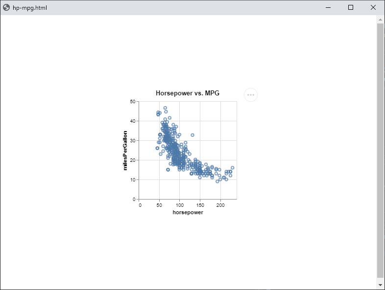
Create a scatter plot specification comparing horsepower and miles per
gallon:
(plot:plot (vega:defplothp-mpg`(:title"Horsepower vs. MPG":description"Horsepower vs miles per gallon for various cars":data (:values,vgcars)
:mark:point:encoding (:x (:field:horsepower:type:quantitative)
:y (:field:miles-per-gallon:type:quantitative)))))
2.1 - Installation
Installing and configuring Lisp-Stat
Intallation methods
Online Notebook
The easiest way to get started is with the link above which will open a preconfigured
notebook on mybinder.org.
Local Jupyter Container
You can also run the Jupyter notebook in a pre-built OCI image. This is a minimal Docker file:
FROM ghcr.io/lisp-stat/cl-jupyter:latest
Our images are based on Jupyter Docker Stacks and all of their
documentation is applicable to the cl-jupyter image.
For a quickstart:
docker run -it -p 8888:8888 ghcr.io/lisp-stat/cl-jupyter:latest
# Entered start.sh with args: jupyter lab# ...# To access the server, open this file in a browser:# file:///home/jovyan/.local/share/jupyter/runtime/jpserver-7-open.html# Or copy and paste one of these URLs:# http://eca4aa01751c:8888/lab?token=d4ac9278f5f5388e88097a3a8ebbe9401be206cfa0b83099# http://127.0.0.1:8888/lab?token=d4ac9278f5f5388e88097a3a8ebbe9401be206cfa0b83099
This command pulls the latest cl-jupyter image from ghcr.io if it is not already present on the local host. It then starts a container running a Jupyter Server with the JupyterLab frontend and exposes the server on host port 8888. The server logs appear in the terminal and include a URL to the server.
Local OCI/Docker
If you prefer a traditional Lisp development environment, there is a ls-dev-image configured with emacs, slime and ls-server for remote data and plotting. A one-liner for getting started there is:
See the README in the repo above for more options and instructions.
Initialization file
You can put customisations to your environment in either your
implementation’s init file, or in a personal init file and load it
from the implementation’s init file. For example, I keep my
customisations in #P"~/ls-init.lisp" and load it from SBCL’s init
file ~/.sbclrc in a Lisp-Stat initialisation section like this:
Settings in your personal lisp-stat init file override the system defaults.
Here’s an example ls-init.lisp file that loads some common R data sets:
(defparameter*default-datasets*'("tooth-growth""plant-growth""usarrests""iris""mtcars")
"Data sets loaded as part of personal Lisp-Stat initialisation.
Available in every session.")
(mapnil#'(lambda (x)
(formatt"Loading ~A~%"x)
(datax))
*default-datasets*)
With this init file, you can immediately access the data sets in the
*default-datasets* list defined above, e.g.:
We assume an experienced user will have their own Emacs and lisp
implementation and will want to install according to their own tastes
and setup. The repo links you need are below, or you can install with
quicklisp.
Prerequisites
All that is needed is an ANSI Common Lisp implementation. Development
is done with SBCL. Other platforms should work, but will
not have been tested, nor can we offer support (maintaining & testing
on multiple implementations requires more resources than the project
has available). Note that CCL is not in good health, and there are a
few numerical bugs that remain unfixed. A shame, as we really liked
CCL.
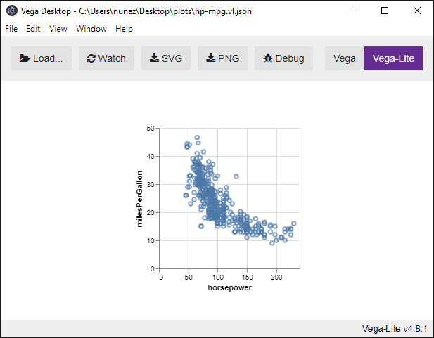
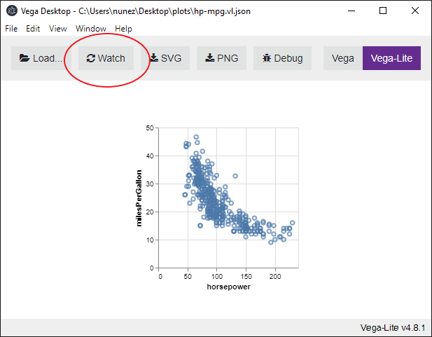
You may want to consider emacs-vega-view
for viewing plots from within emacs.
Installation
The easiest way to install Lisp-Stat is via
Quicklisp, a library manager for
Common Lisp. It works with your existing Common Lisp implementation to
download, install, and load any of over 1,500 libraries with a few
simple commands.
Quicklisp is like a package manager in Linux. It can load packages
from the local file system, or download them if required. If you have
quicklisp installed, you can use:
(ql:quickload:lisp-stat)
Quicklisp is good at managing the project dependency retrieval, but
most of the time we use ASDF because of its REPL integration. You only
have to use Quicklisp once to get the dependencies, then use ASDF for
day-to-day work.
You can install additional Lisp-Stat modules in the same way. For example to install the CEPHES module:
(ql:quickload:cephes)
Loading
Once you have obtained Lisp-Stat via Quicklisp, you can load in one of two ways:
ASDF
Quicklisp
Loading with ASDF
(asdf:load-system:lisp-stat)
If you are using emacs, you can use the slime
shortcuts to
load systems by typing , and then load-system in the mini-buffer.
This is what the Lisp-Stat developers use most often, the shortcuts
are a helpful part of the workflow.
Loading with Quicklisp
To load with Quicklisp:
(ql:quickload:lisp-stat)
Quicklisp uses the same ASDF command as above to load Lisp-Stat.
Updating Lisp-Stat
When a new release is announced, you can update via Quicklisp like so:
(ql:update-dist"lisp-stat")
Documentation
You can install the info manuals into the emacs help system and this
allows searching and browsing from within the editing environment. To
do this, use the
install-info
command. As an example, on my MS Windows 10 machine, with MSYS2/emacs
installation:
installs the select manual at the top level of the info tree. You
can also install the common lisp hyperspec and browse documentation
for the base Common Lisp system. This really is the best way to use
documentation whilst programming Common Lisp and Lisp-Stat. See the
emacs external
documentation
and “How do I install a piece of Texinfo
documentation?”
for more information on installing help files in emacs.
See getting help for
information on how to access Info documentation as you code. This is
the mechanism used by Lisp-Stat developers because you don’t have to
leave the emacs editor to look up function documentation in a browser.
This manual is organised by audience. The overview
and getting started sections are applicable
to all users. Other sections are focused on statistical practitioners,
developers or users new to Common Lisp.
Examples
This part of the documentation contains worked examples of statistical
analysis and plotting. It has less explanatory material, and more
worked examples of code than other sections. If you have a common
use-case and want to know how to solve it, look here.
Tutorials
This section contains tutorials, primers and ‘vignettes’. Typically
tutorials contain more explanatory material, whilst primers are
short-form tutorials on a particular system.
System manuals
The manuals are written at a level somewhere between an API reference
and a core task. (‘annotated reference’) They document, with text and examples, the core APIs
of each system. These are useful references for power users,
developers and if you need to go a bit beyond the core tasks.
Reference
The reference manuals document the API for each system. These are
typically used by developers building extensions to Lisp-Stat.
Resources
Common Lisp and statistical resources, such as books, tutorials and
website. Not specific to Lisp-Stat, but useful for statistical
practitioners learning Lisp.
Contributing
This section describes how to contribute to Lisp-Stat. There are both
ideas on what to contribute, as well as instructions on how to
contribute. Also note the section on the top right of all the
documentation pages, just below the search box:
If you see a mistake in the documentation, please use the Create documentation issue link to go directly to github and report the
error.
2.3 - Getting Help
Ways to get help with Lisp-Stat
There are several ways to get help with Lisp-Stat and your statistical
analysis. This section describes way to get help with your data
objects, with Lisp-Stat commands to process them, and with Common
Lisp.
Search
We use the algolia search engine to index
the site. This search engine is specialised to work well with
documentation websites like this one. If you’re looking for something
and can’t find it in the navigation panes, use the search box:
Apropos
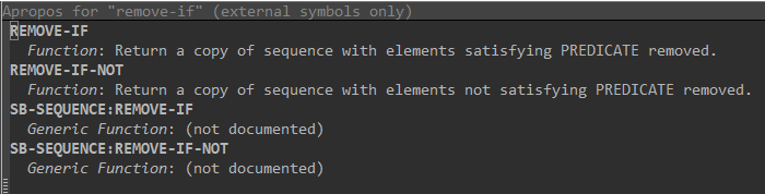
If you’re not quite sure what you’re looking for, you can use the
apropos command. You can do this either from the REPL or hemlock/emacs.
Here are two examples:
If you use the emacs/slime command sequence C-c C-d a, (all the slime documentation commands start with C-c C-d) emacs will ask you for a string. Let’s say you typed in remove-if. Emacs will open a buffer like the one below with all the docs strings for similar functions or variables:
Emacs apropos
Restart from errors
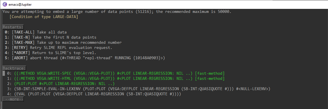
Common lisp has what is called a condition system, which is somewhat unique. One of the features of the condition system is something call restarts. Basically, one part of the system can signal a condition, and another part of it can handle the condition. One of the ways a signal can be handled is by providing various restarts. Restarts happen by the debugger, and many users new to Common Lisp tend to shy away from the debugger (this is common to other languages too). In Common Lisp the debugger is both for developers and users.
Well written Lisp programs will provide a good set of restarts for commonly encountered situations. As an example, suppose we are plotting a data set that has a large number of data points. Experience has shown that greater than 50,000 data points can cause browser performance issues, so we’ve added a restart to warn you, seen below:
Here you can see we have options to take all the data, take n (that the user will provide) or take up to the maximum recommended number. Always look at the options offered to you by the debugger and see if any of them will fix the problem for you.
Describe data
You can use the describe command to print a description of just
about anything in the Lisp environment. Lisp-Stat extends this
functionality to describe data. For example:
LS-USER> (describe'mtcars)
LS-USER::MTCARS[symbol]MTCARSnamesaspecialvariable:Value:#<DATA-FRAME (32observationsof12variables)
MotorTrendCarRoadTests>Documentation:MotorTrendCarRoadTestsDescriptionThedatawasextractedfromthe1974MotorTrendUSmagazine,andcomprisesfuelconsumptionand10aspectsofautomobiledesignandperformancefor32automobiles (1973–74models).NoteHendersonandVelleman (1981) commentinafootnotetoTable1:‘Hocking[originaltranscriber]'snoncrucialcodingoftheMazda'srotaryengineasastraightsix-cylinderengineandthePorsche'sflatengineasaVengine,aswellastheinclusionofthedieselMercedes240D,havebeenretainedtoenabledirectcomparisonstobemadewithpreviousanalyses.’SourceHendersonandVelleman (1981),Buildingmultipleregressionmodelsinteractively.Biometrics,37,391–411.Variables:Variable| Type |Unit| Label
-------- |----| ---- |-----------MODEL| STRING |NIL| NIL
MPG |DOUBLE-FLOAT| M/G |Miles/(US) gallonCYL| INTEGER |NA| Number of cylinders
DISP |DOUBLE-FLOAT| IN3 |Displacement (cu.in.)
HP| INTEGER |HP| Gross horsepower
DRAT |DOUBLE-FLOAT| NA |RearaxleratioWT| DOUBLE-FLOAT |LB| Weight (1000 lbs)
QSEC |DOUBLE-FLOAT| S |1/4miletimeVS| CATEGORICAL |NA| Engine (0=v-shaped, 1=straight)
AM |CATEGORICAL| NA |Transmission (0=automatic,1=manual)
GEAR| CATEGORICAL |NA| Number of forward gears
CARB |CATEGORICAL| NA |Numberofcarburetors
Documentation
The documentation command can be used to read the documentation of a function or variable. Here’s how to read the documentation for the Lisp-Stat mean function:
LS-USER> (documentation'mean'function)
"The mean of elements in OBJECT."
You can also view the documentation for variables or data objects:
LS-USER> (documentation'*ask-on-redefine*'variable)
"If non-nil the system will ask the user for confirmation
before redefining a data frame"
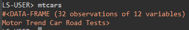
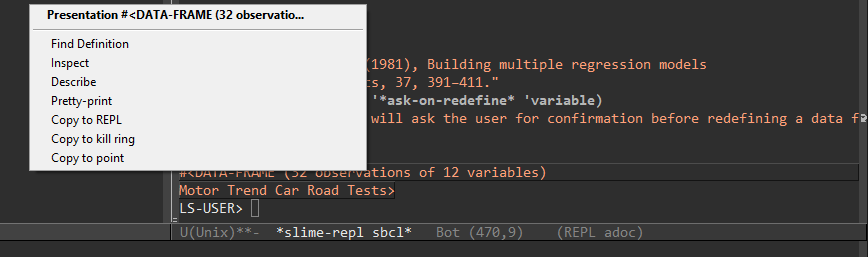
Emacs inspector
When Lisp prints an interesting object to emacs/slime, it will be
displayed in orange text. This indicates that it is a presentation, a
special kind of object that we can manipulate. For example if you type
the name of a data frame, it will return a presentation object:
Now if you right click on this object you’ll get the presentation menu:
From this menu you can go to the source code of the object, inspect &
change values, describe it (as seen above, but within an emacs
window), and copy it.
Slime inspector
The slime
inspector is
an alternative inspector for emacs, with some additional
functionality.
Slime documentation
Slime documentation provides ways to browse documentation from the editor. We saw one example above with apropos. You can also browse variable and function documentation. For example if you have the cursor positioned over a function:
(show-data-frames)
and you type C-c C-d f (describe function at point), you’ll see this
in an emacs window:
#<FUNCTION SHOW-DATA-FRAMES>
  [compiled function]


Lambda-list: (&KEY (HEAD NIL) (STREAM *STANDARD-OUTPUT*))
Derived type: (FUNCTION (&KEY (:HEAD T) (:STREAM T)) *)
Documentation:
  Print all data frames in the current environment in
  reverse order of creation, i.e. most recently created first.
  If HEAD is not NIL, print the first six rows, similar to the
  HEAD function.
Source file: s:/src/data-frame/src/defdf.lisp
Select a name for your new project and click Create repository from template
Make your own local working copy of your new repo using git clone, replacing https://github.com/me/example.git with your
repo’s URL:
git clone --depth 1 https://github.com/me/example.git
You can now edit your own versions of the project’s source files.
This will clone the project template into your own github repository
so you can begin adding your own files to it.
Directory Structure
By convention, we use a directory structure that looks like this:
Often your project will have sample data used for examples
illustrating how to use the system. Such example data goes here, as
would static data files that your system includes, for example post
codes (zip codes). For some projects, we keep the project data here
too. If the data is obtained over the network or a data base, login
credentials and code related to that is kept here. Basically,
anything neccessary to obtain the data should be kept in this
directory.
src
The lisp source code for loading, cleaning and analysing your data.
If you are using the template for a Lisp-Stat add-on package, the
source code for the functionality goes here.
tests
Tests for your code. We recommend CL-UNIT2 for test
frameworks.
docs
Generated documentation goes here. This could be both API
documentation and user guides and manuals. If an index.html file
appears here, github will automatically display it’s contents at
project.github.io, if you have configured the repository to display
documentation that way.
Load your project
If you’ve cloned the project template into your local Common Lisp
directory, ~/common-lisp/, then you can load it with (ql:quickload :project). Lisp will download and compile the necessary
dependencies and your project will be loaded. The first thing you’ll
want to do is to configure your project.
Configure your project
First, change the directory and repository name to suit your
environment and make sure git remotes are working properly. Save
yourself some time and get git working before configuring the project
further.
ASDF
The project.asd file is the Common Lisp system definition file.
Rename this to be the same as your project directory and edit its
contents to reflect the state of your project. To start with, don’t
change any of the file names; just edit the meta data. As you add or
rename source code files in the project you’ll update the file names
here so Common Lisp will know that to compile. This file is analgous
to a makefile in C – it tells lisp how to build your project.
Initialisation
If you need project-wide initialisation settings, you can do this in
the file src/init.lisp. The template sets up a logical path
name for
the project:
To use it, you’ll modify the directories and project name for your
project, and then call (setup-project-translations) in one of your
lisp initialisation files (either ls-init.lisp or .sbclrc). By
default, the project data directory will be set to a subdirectory
below the main project directory, and you can access files there with
PROJECT:DATA;mtcars.csv for example. When you configure your
logical pathnames, you’ll replace “PROJECT” with your projects name.
We use logical style pathnames throughout the Lisp-Stat documentation,
even if a code level translation isn’t in place.
Basic workflow
The project templates illustrates the basic steps for a simple
analysis.
Load data
The first step is to load data. The PROJECT:SRC;load file shows
creating three data frames, from three different sources: CSV, TSV and
JSON. Use this as a template for loading your own data.
Cleanse data
load.lisp also shows some simple cleansing, adding labels, types and
attributes, and transforming (recoding) a variable. You can follow
these examples for your own data sets, with the goal of creating a
data frame from your data.
Analyse
PROJECT:SRC;analyse shows taking the mean and standard deviation of
the mpg variable of the loaded data set. Your own analysis will, of
course, be different. The examples here are meant to indicate the
purpose. You may have one or more files for your analysis, including
supporting functions, joining data sets, etc.
Plot
Plotting can be useful at any stage of the process. It’s inclusion as
the third step isn’t intended to imply a particular importance or
order. The file PROJECT:SRC;plot shows how to plot the information
in the disasters data frame.
Save
Finally, you’ll want to save your data frame after you’ve got it where
you want it to be. You can save project in a ’native’ format, a lisp
file, that will preserve all your meta data and is editable, or a CSV
file. You should only use a CSV file if you need to use the data in
another system. PROJECT:SRC;save containes an example that shows how to save your work.
3 - Examples
Using Lisp-Stat in the real world
One of the best ways to learn Lisp-Stat is to see examples of actual work. This section contains example notebooks illustrating statistical analysis. These notebooks describe how to undertake statistical analyses introduced as examples in the Ninth Edition of Introduction to the Practices of Statistics (2017) by Moore, McCabe and Craig. The notebooks are organised in the same manner as the chapters of the book. The data comes from the site IPS9 in R by Nicholas Horton.
To run the notebooks yourself you can use a ready made online notebook:
Building plots with composable, ggplot-style helper functions
Overview
The geom and gg packages provide a set of composable helper
functions for building Vega-Lite
plot specifications. Inspired by R’s
ggplot2, specifications are
constructed by combining independent layers — geometry, labels, scales,
coordinates and themes — rather than writing monolithic JSON-like
plists by hand.
Each helper returns a plist. The function merge-plists recursively
merges them into a single Vega-Lite spec, which vega:defplot
compiles and plot:plot renders.
Package setup
The examples below
assume you are working in the LS-USER package so you need to use the
qualified forms (geom:point, gg:label, etc.) or import the
appropriate symbols into the current package (which should be
LS-USER):
In ggplot2, a plot is built from independent concerns:
ggplot2
Lisp-Stat
Package
Responsibility
geom_point()
point
geom
Mark type and encoding
geom_bar()
bar
geom
Mark type and encoding
geom_boxplot()
box-plot
geom
Mark type and encoding
geom_histogram()
histogram
geom
Binning, aggregation
geom_line()
line
geom
Series connection, interpolation
labs()
label
gg
Axis titles
scale_*()
axes
gg
Axis transforms, domains, color schemes
coord_cartesian()
coord
gg
Viewport clipping
theme()
theme
gg
Dimensions, fonts, appearance
(no direct equiv.)
tooltip
gg
Hover field definitions
Each function knows about one concern and nothing else. A mark
function never sets axis titles; label never touches mark types;
theme never alters encodings. This separation means any helper can
be used with any plot type.
The merge pattern
Every helper returns a plist fragment. merge-plists performs a
recursive deep merge: when two plists both supply a nested plist for
the same key (e.g. :encoding), the inner plists are merged rather
than one replacing the other. This is what allows label to add
:axis entries to the :encoding that point already created.
Note that merge-plists is a utility function, not a layer helper —
it is the mechanism that makes composition work, not a layer you
pass to qplot yourself. See the API reference for full details.
Two ways to plot
Lisp-Stat provides two entry points for creating plots. Choose the one
that fits your workflow.
defplot + plot:plot — the explicit pattern
The traditional approach separates definition from rendering. Use this
when you want full control, or when writing scripts and notebooks.
Replace :x-field, :y-field, and my-data with your actual field
names and data source:
Registers it in *all-plots* so show-plots can list it
plot:plot then renders the object to the browser.
qplot — quick plot for the REPL
For interactive exploration, the three-line scaffold of plot:plot /
vega:defplot / merge-plists is repetitive. qplot collapses it
into a single function call:
qplot takes a name (a symbol), a data object (a data frame,
plist data, or URI), and any number of layer plists. It:
Prepends (:data (:values ,data)) and merges all layers
Creates the plot object via %defplot
Binds it to the named global variable
Registers it in *all-plots*
Renders immediately via plot:plot
Returns the plot object
Because qplot binds a named variable, the standard REPL workflow is
to re-evaluate the same form as you iterate on a plot. Each call
overwrites the previous definition — there is no accumulation in
*all-plots* or in the global namespace:
;; First attempt — rough sketch(qplot'carsvgcars (point:horsepower:miles-per-gallon))
;; Second attempt — add color and a title(qplot'carsvgcars`(:title"HP vs MPG")
(point:horsepower:miles-per-gallon:color:origin:filledt))
;; Third attempt — polish for presentation(qplot'carsvgcars`(:title"HP vs MPG")
(point:horsepower:miles-per-gallon:color:origin:filledt)
(label:x"Horsepower":y"Fuel Efficiency")
(theme:width600:height400))
;; Later — the variable is still boundcars; => #<VEGA-PLOT ...>(plot:plotcars) ; re-render(describecars) ; inspect the spec(show-plots) ; lists one 'cars' entry
qplot vs defplot
qplot and defplot produce identical plot objects. The only
differences are syntactic: qplot separates the data argument,
handles the merge, and renders immediately. You can freely mix both
styles in the same session — they share *all-plots* and the global
namespace.
Helpers reference
The layering helpers work with all mark types.
label — Set axis titles.
(label:x"Horsepower":y"Miles per Gallon")
axes — Set axis types, domains, ranges, and color schemes.
coord — Restrict the visible viewport and clip marks, like
coord_cartesian() in ggplot2. Only data within the domain is
visible; points outside are clipped rather than dropped.
(coord:x-domain#(50150) :y-domain#(2040))
theme — Set dimensions, font, background, or named presets.
(theme:width600:height400:font"Georgia")
coord vs. axes
axes with :x-domain changes the axis range but does not clip
marks — points outside the domain overflow visibly. coord sets the
domain and clips marks to the viewport, matching coord_cartesian()
semantics. Choose coord when you want to zoom into a region;
choose axes when you want to change the axis transform without
hiding data.
Vectors for JSON arrays
Vega-Lite expects JSON arrays for domain, range, tooltip, and
similar properties. In the JSON serializer, lists become JSON
objects and vectors become JSON arrays. Always use #(...) or
(vector ...) when you need a JSON array:
Field names are passed as keywords (e.g. :horsepower,
:origin), not strings. The helpers convert keywords to the
camelCase Vega-Lite field names automatically. Only human-readable
labels — axis titles, plot titles, descriptions — are strings.
;; Correct — keywords for fields, strings for labels(point:horsepower:miles-per-gallon:color:origin)
(label:x"Engine Horsepower":y"Fuel Efficiency")
;; Wrong — strings for field names(point:horsepower:miles-per-gallon:color"origin")
Keywords vs. strings for color values
The :color parameter accepts both keywords and strings, but they
mean different things:
Keyword → a data field mapped to the color encoding channel.
Each unique value in the field gets a distinct hue.
String → a literal CSS color applied directly to the mark.
;; Keyword — map the :origin field to color (encoding)(point:horsepower:miles-per-gallon:color:origin)
;; String — paint every point teal (mark property)(point:horsepower:miles-per-gallon:color"teal")
;; Same convention applies to all mark types(histogram:miles-per-gallon:color:origin) ; stacked by origin(histogram:miles-per-gallon:color"darkslategray") ; uniform bar color(bar:origin:miles-per-gallon:color"teal") ; uniform bar color
This convention is consistent across all mark helpers (point,
bar, histogram, box-plot, line) and all visual channel
parameters (:color, :size, :opacity, etc.): keywords are
field names, strings are literal values.
Loading example data
The examples below use datasets from the Vega datasets collection.
Load them into your session before running the examples:
(vega:load-vega-examples)
This makes the following variables available in your environment:
stocks — Daily closing prices for several major tech stocks over multiple years.
For datasets loaded using vega:read-vega, field names are
automatically converted to Lisp-style keywords (e.g.
Miles_per_Gallon becomes :miles-per-gallon). Note that the
:year field in vgcars is stored as a date string (e.g.
"1970-01-01") rather than an integer, which is why the line chart
examples pass :x-type :temporal for that field.
Scatter plot
A scatter plot maps two quantitative variables to x and y positions.
Use point for exploring relationships, correlations and clusters in
data. The name follows the ggplot2 convention where geom_point()
produces a scatter plot.
Basic scatter plot
The simplest scatter plot needs just a name, a data frame, and two
field names:
(qplot'cars-basicvgcars`(:title"Horsepower vs. MPG")
(point:horsepower:miles-per-gallon))
Color by category
Pass a keyword to :color to map a nominal variable to hue. Use
:filled t to fill the point marks:
(qplot'cars-coloredvgcars`(:title"Cars by Origin")
(point:horsepower:miles-per-gallon:color:origin:filledt))
Bubble plot
When :size is a keyword, it encodes a third quantitative field as
point area — a bubble plot:
(qplot'cars-bubblevgcars`(:title"Bubble: Size = Acceleration")
(point:horsepower:miles-per-gallon:color:origin:size:acceleration:filledt)
(label:x"Horsepower":y"Miles per Gallon"))
A LOESS (locally estimated scatterplot smoothing) curve fits a
non-parametric smooth line through data, revealing trends without
assuming a fixed functional form. Use loess to overlay a trend
line on a scatter plot or to compare smoothed trajectories across
groups.
Scatter plot with LOESS smoother
Use gg:layer to compose the scatter points and the smoother into
a single layered view:
(qplot'cars-loessvgcars`(:title"HP vs. MPG with LOESS Smoother")
(gg:layer (point:horsepower:miles-per-gallon:color:origin:filledt:opacity0.5)
(loess:horsepower:miles-per-gallon:group:origin:stroke-width2)))
The :group :origin argument fits a separate curve for each origin
and encodes it with the matching hue automatically. Increase
:bandwidth toward 1.0 for a flatter, more global fit; decrease
it toward 0.05 for a curve that tracks local variation closely.
Histogram
A histogram bins a quantitative variable and counts observations per
bin. Use histogram to visualize the distribution of a single
variable.
Basic histogram
Pass a single field name. The default uses Vega-Lite’s automatic
binning and counts occurrences:
(qplot'mpg-histvgcars`(:title"Distribution of Miles per Gallon")
(histogram:miles-per-gallon)
(label:x"Miles per Gallon":y"Count"))
Custom bin count
Control granularity with the :bin keyword. Pass a plist with
:maxbins to limit the number of bins:
(qplot'mpg-hist-binsvgcars`(:title"MPG Distribution (10 bins)")
(histogram:miles-per-gallon:bin'(:maxbins10))
(label:x"Miles per Gallon":y"Count"))
Horizontal histogram
Set :orient :horizontal to place bins on the y-axis:
(qplot'mpg-hist-horizvgcars`(:title"MPG Distribution (Horizontal)")
(histogram:miles-per-gallon:orient:horizontal)
(label:x"Count":y"Miles per Gallon"))
Stacked histogram by group
Pass :group to split bins by a nominal field. Vega-Lite
automatically stacks the bars:
(qplot'mpg-hist-stackedvgcars`(:title"MPG Distribution by Origin")
(histogram:miles-per-gallon:group:origin)
(label:x"Miles per Gallon":y"Count"))
Layered histogram
Use :stack :null with :opacity to overlay distributions
transparently instead of stacking them:
(qplot'mpg-hist-layeredvgcars`(:title"MPG: Overlaid by Origin")
(histogram:miles-per-gallon:group:origin:stack:null:opacity0.5)
(label:x"Miles per Gallon":y"Count"))
Normalized (100%) stacked histogram
Use :stack :normalize to show proportions instead of counts:
(qplot'mpg-hist-normalizedvgcars`(:title"MPG: Proportion by Origin")
(histogram:miles-per-gallon:group:origin:stack:normalize)
(label:x"Miles per Gallon":y"Proportion"))
Styled histogram
Use :color, :corner-radius-end, and :bin-spacing for visual
polish. Combine with theme for custom dimensions:
(qplot'mpg-hist-styledvgcars`(:title"Styled Histogram")
(histogram:miles-per-gallon:color"darkslategray":corner-radius-end3:bin-spacing0)
(label:x"Miles per Gallon":y"Count")
(theme:width500:height300))
Bar chart
A bar chart maps a categorical variable to position and a
quantitative variable to bar length. Use bar when your x-axis is
nominal or ordinal rather than a continuous distribution. The name
follows the ggplot2 convention where geom_bar() produces a bar
chart.
Basic bar chart
Supply the categorical field and the quantitative field:
(qplot'origin-barvgcars`(:title"Average MPG by Origin")
(bar:origin:miles-per-gallon:aggregate:mean)
(label:x"Origin":y"Mean Miles per Gallon"))
Horizontal bar chart
Set :orient :horizontal to swap axes — useful for long category
labels:
(qplot'origin-bar-horizvgcars`(:title"Average MPG by Origin (Horizontal)")
(bar:origin:miles-per-gallon:aggregate:mean:orient:horizontal)
(label:x"Mean Miles per Gallon":y"Origin"))
Grouped (stacked) bar chart
Pass :group to split bars by a second nominal field. Bars are
stacked by default:
(qplot'cylinders-by-originvgcars`(:title"Car Count: Cylinders by Origin")
(bar:cylinders:miles-per-gallon:aggregate:count:group:origin)
(label:x"Cylinders":y"Count"))
Styled bar chart
Combine visual options with layering helpers:
(qplot'origin-bar-styledvgcars`(:title"Mean MPG by Origin")
(bar:origin:miles-per-gallon:aggregate:mean:color"teal":corner-radius-end4)
(label:x"Origin":y"Mean MPG")
(theme:width400:height300:font"Helvetica"))
Box plot
A box plot summarizes the distribution of a quantitative variable,
showing the median, interquartile range and outliers. Use box-plot
to compare distributions across groups.
1D box plot
A single quantitative field produces a box plot summarizing the
entire variable:
(qplot'mpg-box-1dvgcars`(:title"MPG Distribution")
(box-plot:miles-per-gallon)
(label:x"Miles per Gallon"))
2D box plot — compare groups
Pass :category to split the box plot by a nominal field:
(qplot'mpg-box-by-originvgcars`(:title"MPG by Origin")
(box-plot:miles-per-gallon:category:origin)
(label:x"Miles per Gallon":y"Origin"))
Vertical orientation
Set :orient :vertical to place categories on the x-axis and values
on the y-axis:
(qplot'mpg-box-verticalvgcars`(:title"MPG by Cylinders (Vertical)")
(box-plot:miles-per-gallon:category:cylinders:orient:vertical)
(label:x"Cylinders":y"Miles per Gallon"))
Min-max whiskers
Set :extent "min-max" to extend whiskers to the minimum and
maximum values instead of the default 1.5× IQR (Tukey) whiskers:
(qplot'mpg-box-minmaxvgcars`(:title"MPG by Origin (Min-Max Whiskers)")
(box-plot:miles-per-gallon:category:origin:extent"min-max") ; note string value (label:x"Miles per Gallon":y"Origin"))
Styled box plot
Combine visual options with layering helpers for presentation:
(qplot'mpg-box-styledvgcars`(:title"MPG by Origin")
(box-plot:miles-per-gallon:category:origin:orient:vertical:size40)
(label:x"Origin":y"Miles per Gallon")
(theme:width500:height350))
Line chart
A line chart connects data points in order, typically along a
temporal or sequential x-axis. Use line for time series, trends,
and any data where the relationship between consecutive points is
meaningful. The name follows the ggplot2 convention where
geom_line() produces a line chart.
Basic line chart
The simplest line chart needs two field names. Points are connected
in x-axis order:
Pass a keyword to :color to draw a separate line for each
category:
(qplot'stock-coloredstocks`(:title"Stock Prices by Company")
(line:date:price:color:symbol:x-type:temporal)
(label:x"Date":y"Price (USD)"))
Smoothed interpolation
Set :interpolate to control how points are connected. Common
values are :linear (default), :monotone (smooth, monotonic
curves), :step (step function), :basis (B-spline), and
:cardinal:
Set :point t to overlay point marks on each data position — useful
for sparse data or when exact values matter. Note that :x-type :temporal is required here because the :year field in vgcars is
stored as a date string rather than an integer:
(qplot'mpg-trendvgcars`(:title"Mean MPG by Model Year")
(line:year:miles-per-gallon:pointt:x-type:temporal)
(label:x"Model Year":y"Miles per Gallon"))
Use :interpolate :step for piecewise-constant lines — useful for
data that changes at discrete intervals (e.g. interest rates,
pricing tiers):
(qplot'mpg-stepvgcars`(:title"MPG by Year (Step)")
(line:year:miles-per-gallon:interpolate:step:x-type:temporal)
(label:x"Model Year":y"Miles per Gallon"))
Styled multi-series line chart
Combine all options with layering helpers for a polished
presentation:
(qplot'stock-fullstocks`(:title"Stock Comparison":description"Daily closing prices for major tech stocks")
(line:date:price:color:symbol:interpolate:monotone:stroke-width2:x-type:temporal)
(label:x"Date":y"Closing Price (USD)")
(axes:color-scheme:dark2)
(tooltip'(:field:symbol:type:nominal)
'(:field:date:type:temporal)
'(:field:price:type:quantitative))
(theme:width700:height400))
Function curves
geom:func plots a Lisp function as a smooth line by evaluating it at
evenly-spaced sample points and embedding the resulting (x, y) pairs
directly in the Vega-Lite specification. It mirrors the behaviour of
R’s geom_function()
from ggplot2.
Unlike the data-driven helpers (point, bar, histogram, etc.),
func is self-contained: it carries its own :data block and
requires no external data frame. Use it anywhere you want to visualise
a mathematical relationship — probability densities, regression curves,
physical models, or any other computable function.
Import func alongside the other helpers you use:
(import'(geom:func))
How it works
func calls aops:linspace to generate n evenly-spaced x values
over the closed interval [xmin, xmax] specified by :xlim. It
then calls fn at each x, collects the (x, y) pairs into a vector
of plists, and embeds them as an inline Vega-Lite :data block.
A :line mark connects the points using the chosen interpolation
method (:monotone by default, giving smooth curves without
overshoot).
Points where fn signals a condition (e.g. (log 0), (/ 1 0))
or returns a non-finite value (± infinity, NaN) are silently
dropped. Vega-Lite renders a visible gap at each discontinuity —
the correct visual for functions like tan or 1/x.
Design note: self-contained data
All other geom helpers return only :mark and :encoding keys and
rely on the caller to supply :data. func also returns a :data
key, because the data is the function. This means it composes
slightly differently from the other geom helpers:
Helper
Data source
Typical entry point
point, bar, histogram, …
external data frame
qplot
func
self-generated inline
defplot + vega:merge-plists
For multi-layer plots (function overlaid on data) use Vega-Lite’s
:layer array directly inside defplot; see
Overlay on scatter data below.
The following table describes the ggplot2 equivalent and responsibility:
ggplot2
Lisp-Stat
Package
Responsibility
geom_function()
func
geom
Sample a function, encode as a line
Reference
(geom:func fn &key xlim n color stroke-width stroke-dash opacity interpolate)
Parameter
Type
Default
Description
fn
function
—
A Lisp function (real → real). Receives a double-float; must return a real.
:xlim
vector
#(0d0 1d0)
Domain #(xmin xmax). Both endpoints are always sampled.
:n
integer ≥ 2
100
Number of sample points. Increase for oscillatory functions.
:color
string
nil
CSS color for the line, e.g. "steelblue" or "#e63946". nil lets Vega-Lite choose.
:stroke-width
number
nil
Line thickness in pixels.
:stroke-dash
vector
nil
Dash/gap pattern, e.g. #(6 3) for dashes or #(2 2) for dots.
:opacity
number 0–1
nil
Line opacity.
:interpolate
keyword
:monotone
Vega-Lite interpolation method. :linear, :basis, :cardinal, :step are also accepted.
Vectors for JSON arrays
:xlim and :stroke-dash must be vectors (e.g. #(0 10)), not
lists. In the JSON serializer, lists become JSON objects while
vectors become JSON arrays.
color is always a CSS string
Unlike the other mark helpers, func does not support a keyword
:color for field-based color encoding — a function curve is a single
computed series and carries no nominal grouping field. :color always
takes a CSS color string (e.g. "steelblue").
Top-level :data in layer specs
vega:defplot always validates the top-level :data key. In a
:layer plot where every layer is self-contained (as all func
layers are), pass :data (:values #()) as a placeholder. Vega-Lite
discards it when each layer declares its own :data. This same
placeholder is needed for any defplot form that uses :layer
without shared top-level data.
Basic function plot
Supply a function and a domain. vega:merge-plists combines the
self-contained func layer with a title and axis labels:
Points where fn raises a condition or returns ±infinity are silently
dropped. Vega-Lite draws a gap at each discontinuity — the correct
rendering for functions like tan(x):
(vega:defplottangent-curve (vega:merge-plists`(:title"tan(x) — gaps at singularities")
(func#'tan:xlim#(-4.54.5) :n500)
(label:x"x":y"tan(x)")
(axes:y-domain#(-1010))))
Controlling the visible range
For functions with large excursions near a singularity, use axes
with :y-domain to restrict the visible range. Unlike coord,
axes changes the axis extent without clipping the line marks, which
avoids visual artefacts near the asymptotes.
Probability density function
Plot a probability density function using the distributions system.
Load it before running these examples:
(asdf:load-system:distributions)
Create a distribution object with distributions:r-normal, then pass
its pdf method to func. r-normal takes mean and
variance (not standard deviation), so the standard normal is
(r-normal 0d0 1d0):
distributions:r-normal is parameterised as (r-normal mean variance).
To construct a distribution from a standard deviation sigma, pass
(expt sigma 2) as the second argument. Passing sigma directly
will produce a distribution with the wrong spread and no error.
Styled function curve
Pass :color, :stroke-width, and :stroke-dash for visual polish.
To show two styled curves together, use :layer — each func call
carries its own inline data:
(vega:defplotsin-and-cos-styled`(:title"sin and cos — styled lines":data (:values#())
:layer#(,(func#'sin:xlim#(-6.2836.283)
:n200:color"steelblue":stroke-width2)
,(func#'cos:xlim#(-6.2836.283)
:n200:color"firebrick":stroke-width2:stroke-dash#(84)))))
Step interpolation
Use :interpolate :step for piecewise-constant functions — useful for
visualising floor, ceiling, or any discrete-valued function:
When using :layer directly, add axis titles inside each layer’s
:encoding entry, or use the top-level :encoding key for shared
axes — Vega-Lite will merge them automatically. Alternatively, wrap
the :layer spec in vega:merge-plists and add a label layer
at the outer level.
Family of curves
Plot a parameterised family by building the :layer vector in a loop:
When overlaying a function on top of data, each layer supplies its own
:data. The data layer uses the original data frame; the function
layer uses the inline data generated by func:
(vega:defplotcars-with-trend`(:title"HP vs MPG with Quadratic Trend":data (:values#())
:layer#(;; Layer 1: raw data as a scatter plot (:data (:values,vgcars)
:mark (:type:point:filledt:opacity0.5)
:encoding (:x (:field:horsepower:type:quantitative:title"Horsepower")
:y (:field:miles-per-gallon:type:quantitative:title"Miles per Gallon")
:color (:field:origin:type:nominal)))
;; Layer 2: fitted quadratic y = 52 - 0.23x + 3e-4*x^2,(func (lambda (x)
(+52.0d0 (*-0.23d0x)
(*3.0d-4 (exptx2))))
:xlim#(40230)
:n300:color"firebrick":stroke-width2.5))))
Field names in overlay plots
The function layer always uses the internal field names :x and :y.
The data layer uses the actual field names from your data frame (e.g.
:horsepower, :miles-per-gallon). Vega-Lite resolves the axis
scales across layers automatically when the quantitative ranges
overlap, which is why the function curve aligns correctly with the
scatter points.
Normal distribution fit over a histogram
Overlay the theoretical PDF on an empirical histogram. Use
select:select to extract the column as a vector, statistics:sd
for the standard deviation, and distributions:r-normal to construct
the fitted distribution — recall that r-normal takes the variance,
so pass (expt sigma 2):
(let* ((mpg (select:selectvgcarst:miles-per-gallon))
(mu (statistics:meanmpg))
(sigma (statistics:sdmpg))
(d (distributions:r-normalmu (exptsigma2))))
(vega:defplotmpg-fit`(:title"MPG: Empirical Histogram with Normal Fit":data (:values#())
:layer#(;; Histogram layer (:data (:values,vgcars)
:mark:bar:encoding (:x (:field:miles-per-gallon:bin (:maxbins15)
:type:quantitative:title"Miles per Gallon")
:y (:aggregate:count:stack:null:type:quantitative:title"Count")))
;; Density curve — scaled by (n × bin-width) to match count axis,(func (lambda (x) (*4063 (distributions:pdfdx)))
:xlim#(550)
:n300:color"firebrick":stroke-width2)))))
Chebyshev approximation
numerical-utilities provides chebyshev-regression and
evaluate-chebyshev for polynomial approximation. Plot the exact
function and its approximation together to inspect accuracy:
Because every helper returns an independent plist, you can mix and
match freely. Here are patterns that work with all mark types.
Labels on any plot
label works identically on every plot type — it only touches
:encoding :x/:y :axis :title. The examples below produce the same
visual results as the per-section examples above; they are shown here
to illustrate that label requires no changes across mark types:
;; On a scatter plot(qplot'point-labeledvgcars (point:horsepower:miles-per-gallon)
(label:x"Engine Horsepower":y"Fuel Efficiency"))
;; On a histogram(qplot'hist-labeledvgcars (histogram:horsepower)
(label:x"Engine Horsepower":y"Number of Cars"))
;; On a bar chart(qplot'bar-labeledvgcars (bar:origin:miles-per-gallon:aggregate:mean)
(label:x"Country of Origin":y"Average MPG"))
;; On a box plot(qplot'box-labeledvgcars (box-plot:miles-per-gallon:category:origin)
(label:x"Fuel Efficiency":y"Manufacturing Origin"))
Theme on any plot
theme sets top-level properties that apply to every plot type:
coord works best with quantitative (continuous) axes. For bar
charts and box plots whose axes are categorical, use coord with
:clip nil to avoid cutting marks, or use axes with :x-domain
or :y-domain instead:
;; Zoom a scatter plot — clip marks outside the viewport(coord:x-domain#(50150) :y-domain#(2040))
;; Restrict a bar chart's quantitative axis — no clipping(coord:y-domain#(035) :clipnil)
;; Alternatively, use axes for categorical axes(axes:y-domain#(035))
Recipe: exploring a new dataset
When you first load a dataset, a quick exploratory sequence might
look like this. Note how the same plot name can be reused — each
qplot call overwrites the previous definition.
Step 1 — Distribution of a key variable
Start with a histogram to understand the shape of the data:
(qplot'explore-2vgcars`(:title"HP vs. MPG")
(point:horsepower:miles-per-gallon:filledt))
Step 3 — Compare groups
Break the data down by category to see if patterns differ:
(qplot'explore-3vgcars`(:title"MPG by Origin")
(box-plot:miles-per-gallon:category:origin:orient:vertical)
(label:x"Origin":y"MPG"))
Step 4 — Add detail
Color by group and add labels to confirm the story:
(qplot'explore-4vgcars`(:title"HP vs. MPG by Origin")
(point:horsepower:miles-per-gallon:color:origin:filledt)
(label:x"Horsepower":y"Miles per Gallon")
(tooltip'(:field:name:type:nominal)
'(:field:origin:type:nominal)
'(:field:horsepower:type:quantitative)
'(:field:miles-per-gallon:type:quantitative)))
At the REPL, every call overwrites the same explore variable.
The variable always holds the latest version:
explore; => #<VEGA-PLOT ...>(show-plots) ; one entry for EXPLORE
Tip
For the tutorial we use distinct plot names (explore-1 through
explore-4) so all four plots render on the page. At the REPL you
would reuse 'explore for all of them — only the latest version
is kept.
Recipe: presentation-ready plot
For reports or publications, combine all the layering helpers:
(qplot'presentationvgcars`(:title"Automobile Performance by Country of Origin":description"Horsepower vs fuel efficiency for 406 cars")
(point:horsepower:miles-per-gallon:color:origin:filledt)
(label:x"Engine Horsepower":y"Fuel Efficiency (MPG)")
(axes:color-scheme:tableau10)
(tooltip'(:field:name:type:nominal)
'(:field:horsepower:type:quantitative)
'(:field:miles-per-gallon:type:quantitative))
(theme:width700:height450:font"Helvetica"))
Recipe: saving a plot for later
Once you are happy with a plot created via qplot, it is a
first-class vega-plot object. You can re-render, inspect, or
write it to a file. This example assumes presentation was created
in the recipe above:
;; Re-render in the browser(plot:plotpresentation)
;; Inspect the spec(describepresentation)
;; List all named plots(show-plots)
Recipe: exploring a function
A typical REPL workflow when investigating a mathematical function.
Note how the same plot name is reused — each defplot call overwrites
the previous definition.
Overlay multiple fitted curves on a scatter plot to compare competing
models visually:
(let* ((linear (lambda (x) (+39.9 (*-0.158x))))
(quadratic (lambda (x) (+52.0 (*-0.23x) (*3.0e-4 (exptx2))))))
(vega:defplotmodel-comparison`(:title"Linear vs Quadratic Fit":data (:values#())
:layer#(;; Raw data (:data (:values,vgcars)
:mark (:type:point:filledt:color"lightgray")
:encoding (:x (:field:horsepower:type:quantitative:title"Horsepower")
:y (:field:miles-per-gallon:type:quantitative:title"Miles per Gallon")))
;; Linear fit,(funclinear:xlim#(40230) :n200:color"steelblue":stroke-width2)
;; Quadratic fit,(funcquadratic:xlim#(40230) :n200:color"firebrick":stroke-width2:stroke-dash#(63))))))
Recipe: dropping down to raw Vega-Lite
The helpers cover common patterns. When you need something they
don’t support — transforms, selections, parameters, calculated
fields, multi-view compositions — you can write raw Vega-Lite
directly.
Example: brush selection with linked data table
This example reproduces the
Vega-Lite brush table:
drag a rectangle over the scatter plot to see the selected cars in a
table. It uses hconcat (side-by-side views), params (interactive
brush), and transform (filter + rank) — none of which the helpers
generate. For specs this complex, write the full Vega-Lite plist and
use defplot directly:
(plot:plot (vega:defplotbrush-table`(:description"Drag a rectangular brush to show selected points in a table.":data (:values,vgcars)
:transform#((:window#((:op:row-number:as"row_number"))))
:hconcat#(;; Left panel: scatter plot with brush (:params#((:name"brush":select"interval"))
:mark:point:encoding (:x (:field:horsepower:type:quantitative)
:y (:field:miles-per-gallon:type:quantitative)
:color (:condition (:param"brush":field:cylinders:type:ordinal)
:value"grey")))
;; Right panel: table of selected points (:transform#((:filter (:param"brush"))
(:window#((:op:rank:as"rank")))
(:filter (:field"rank":lt20)))
:hconcat#((:width50:title"Horsepower":mark:text:encoding (:text (:field:horsepower:type:nominal)
:y (:field"row_number":type:ordinal:axis:null)))
(:width50:title"MPG":mark:text:encoding (:text (:field:miles-per-gallon:type:nominal)
:y (:field"row_number":type:ordinal:axis:null)))
(:width50:title"Origin":mark:text:encoding (:text (:field:origin:type:nominal)
:y (:field"row_number":type:ordinal:axis:null))))))
:resolve (:legend (:color:independent)))))
This plot cannot be built with qplot and the layering helpers;
the hconcat layout requires two independent views with different
marks, encodings, and transforms. The rule of thumb:
Use qplot + helpers for single-view plots (scatter, line,
bar, histogram, box plot) with standard encodings
Use defplot + raw plists for multi-view layouts (hconcat,
vconcat, layer, facet), complex interactions, or any
Vega-Lite feature the helpers don’t cover
Both approaches produce the same vega-plot objects and coexist
in the same session.
4.2 - Vega Plotting
Example plots using the vega-lite DSL.
The plots here show equivalents to the Vega-Lite example
gallery. Before you begin working with these example, be certain to read the plotting tutorial where you will learn the basics of working with plot specifications and data.
Preliminaries
Load Vega-Lite
Load Vega-Lite and network libraries:
(asdf:load-system:plot/vega)
and change to the Lisp-Stat user package:
(in-package:ls-user)
Load example data
The examples in this section use the vega-lite data sets. Load them all now:
(vega:load-vega-examples)
Bar charts
Bar charts are used to display information about categorical variables.
Simple bar chart
In this simple bar chart example we’ll demonstrate using literal
embedded data in the form of a plist. Later you’ll see how to use a data-frame directly.
This example uses Seattle weather from the Vega website. Load it into
a data frame like so:
(defdfseattle-weather (read-csvvega:seattle-weather))
;=> #<DATA-FRAME (1461 observations of 6 variables)>
We’ll use a data-frame as the data source via the Common Lisp
backquote
mechanism.
The spec list begins with a backquote (`) and then the data frame is
inserted as a literal value with a comma (,). We’ll use this
pattern frequently.
(plot:plot (vega:defplotstacked-bar-chart`(:mark:bar:data (:values,seattle-weather)
:encoding (:x (:time-unit:month:field:date:type:ordinal:title"Month of the year")
:y (:aggregate:count:type:quantitative)
:color (:field:weather:type:nominal:title"Weather type":scale (:domain#("sun""fog""drizzle""rain""snow")
:range#("#e7ba52","#c7c7c7","#aec7e8","#1f77b4","#9467bd")))))))
Population pyramid
Vega calls this a diverging stacked bar
chart.
It is a population pyramid for the US in 2000, created using the
stack feature of
vega-lite. You could also create one using
concat.
First, load the population data if you haven’t done so:
(defdfpopulation (vega:read-vegavega:population))
;=> #<DATA-FRAME (570 observations of 4 variables)>
Note the use of read-vega in this case. This is because the data in
the Vega example is in an application specific JSON format (Vega, of
course).
Use a relative frequency histogram to compare data sets with different
numbers of observations.
The data is binned with first transform. The number of values per bin
and the total number are calculated in the second and the third
transform to calculate the relative frequency in the last
transformation step.
(plot:plot (vega:defplotstacked-density`(:title"Distribution of Body Mass of Penguins":width400:height80:data (:values,penguins)
:mark:bar:transform#((:density|BODY-MASS-(G)|:groupby#(:species)
:extent#(25006500)))
:encoding (:x (:field:value:type:quantitative:title"Body Mass (g)")
:y (:field:density:type:quantitative:stack:zero)
:color (:field:species:type:nominal)))))
Note the use of the multiple escape
characters
(|) surrounding the field BODY-MASS-(G). This is required because
the JSON data set has parenthesis in the variable names, and these are
reserved characters in Common Lisp. The JSON importer wrapped these
in the escape character.
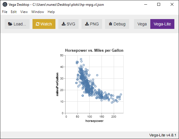
(plot:plot (vega:defplothp-mpg`(:title"Horsepower vs. MPG":data (:values,vgcars)
:mark:point:encoding (:x (:field:horsepower:type"quantitative")
:y (:field:miles-per-gallon:type"quantitative")))))
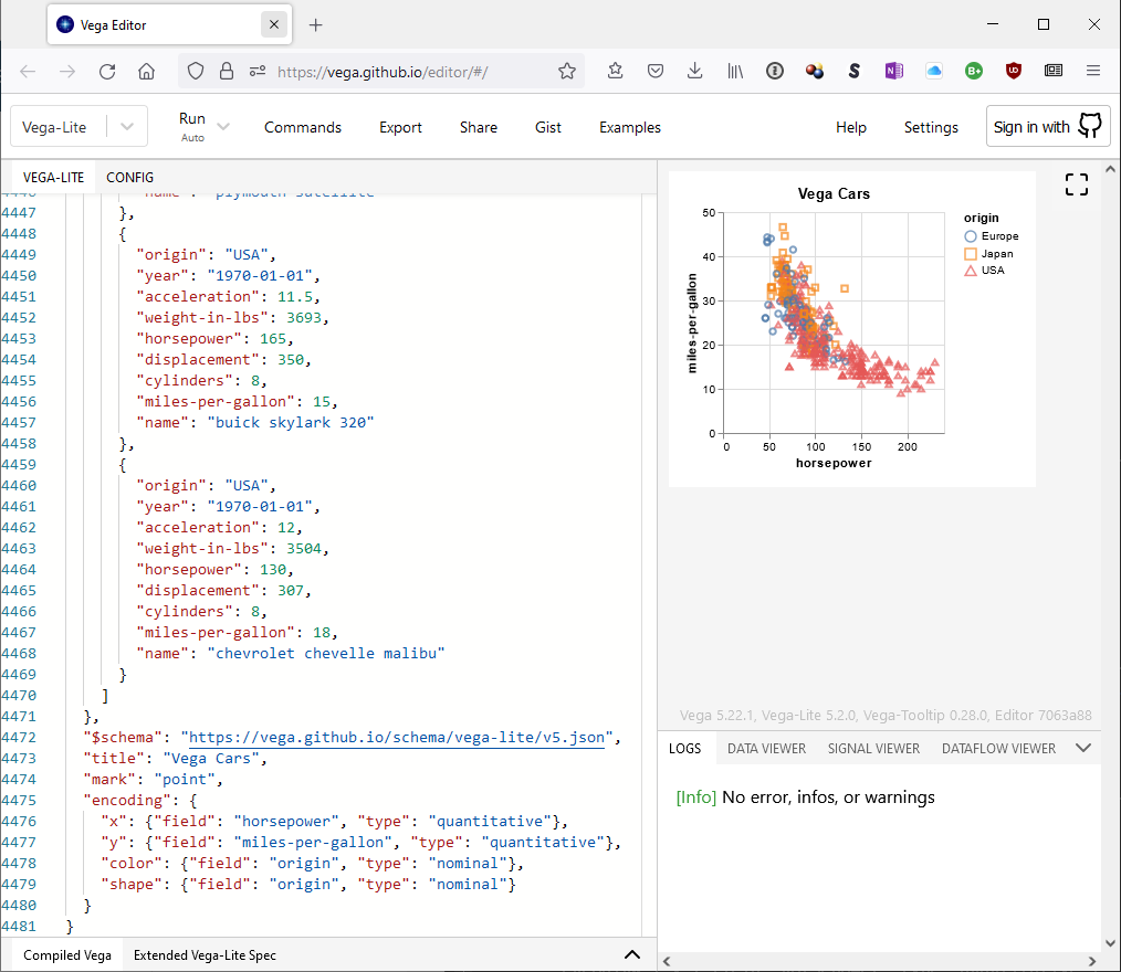
Colored
In this example we’ll show how to add additional information to
the cars scatter plot to show the cars origin. The Vega-Lite
example
shows that we have to add two new directives to the encoding of the
plot:
Notice here we use a string for the field value and not a symbol.
This is because Vega is case sensitive, whereas Lisp is not. We could
have also used a lower-case :as value, but did not to highlight this
requirement for certain Vega specifications.
A dot plot showing each film in the database, and the difference from
the average movie rating. The display is sorted by year to visualize
everything in sequential order. The graph is for all films before
2019. Note the use of the filter-rows function.
The cars scatterplot allows you to see miles per gallon
vs. horsepower. By adding sliders, you can select points by the
number of cylinders and year as well, effectively examining 4
dimensions of data. Drag the sliders to highlight different points.
(plot:plot (vega:defplotnatural-disaster-deaths`(:title"Deaths from global natural disasters":width600:height400:data (:values,(filter-rowsdisasters'(not (string=entity"All natural disasters"))))
:mark (:type:circle:opacity0.8:stroke:black:stroke-width1)
:encoding (:x (:field:year:type:temporal:axis (:grid:false))
:y (:field:entity:type:nominal:axis (:title""))
:size (:field:deaths:type:quantitative:title"Annual Global Deaths":legend (:clip-height30)
:scale (:range-max5000))
:color (:field:entity:type:nominal:legendnil)))))
Note how we modified the example by using a lower case entity in the
filter to match our default lower case variable names. Also note how
we are explicit with parsing the year field as a temporal column.
This is because, when creating a chart with inline data, Vega-Lite
will parse the field as an integer instead of a date.
Line plots
Simple
(plot:plot (vega:defplotsimple-line-plot`(:title"Google's stock price from 2004 to early 2010":data (:values,(filter-rowsstocks'(string=symbol"GOOG")))
:mark:line:encoding (:x (:field:date:type:temporal)
:y (:field:price:type:quantitative)))))
Point markers
By setting the point property of the line mark definition to an object
defining a property of the overlaying point marks, we can overlay
point markers on top of line.
(plot:plot (vega:defplotpoint-mark-line-plot`(:title"Stock prices of 5 Tech Companies over Time":data (:values,stocks)
:mark (:type:line:pointt)
:encoding (:x (:field:date:time-unit:year)
:y (:field:price:type:quantitative:aggregate:mean)
:color (:field:symbol:typenominal)))))
Multi-series
This example uses the custom symbol encoding for variables to
generate the proper types and labels for x, y and color channels.
(plot:plot (vega:defplotmulti-series-line-chart`(:title"Stock prices of 5 Tech Companies over Time":data (:values,stocks)
:mark:line:encoding (:x (:fieldstocks:date)
:y (:fieldstocks:price)
:color (:fieldstocks:symbol)))))
Step
(plot:plot (vega:defplotstep-chart`(:title"Google's stock price from 2004 to early 2010":data (:values,(filter-rowsstocks'(string=symbol"GOOG")))
:mark (:type:line:interpolate"step-after")
:encoding (:x (:fieldstocks:date)
:y (:fieldstocks:price)))))
Stroke-dash
(plot:plot (vega:defplotstroke-dash`(:title"Stock prices of 5 Tech Companies over Time":data (:values,stocks)
:mark:line:encoding (:x (:fieldstocks:date)
:y (:fieldstocks:price)
:stroke-dash (:fieldstocks:symbol)))))
Confidence interval
Line chart with a confidence interval band.
(plot:plot (vega:defplotline-chart-ci`(:data (:values,vgcars)
:encoding (:x (:field:year:time-unit:year))
:layer#((:mark (:type:errorband:extent:ci)
:encoding (:y (:field:miles-per-gallon:type:quantitative:title"Mean of Miles per Gallon (95% CIs)")))
(:mark:line:encoding (:y (:field:miles-per-gallon:aggregate:mean)))))))
This radial plot uses both angular and radial extent to convey
multiple dimensions of data. However, this approach is not
perceptually effective, as viewers will most likely be drawn to the
total area of the shape, conflating the two dimensions. This example
also demonstrates a way to add labels to circular plots.
Normally data transformations should be done in Lisp-Stat with a data
frame. These examples illustrate how to accomplish transformations
using Vega-Lite. This might be useful if, for example, you’re serving
up a lot of plots and want to move the processing to the users
browser.
Difference from avg
(plot:plot (vega:defplotdifference-from-average`(:data (:values,(filter-rowsimdb'(not (eqlimdb-rating:na))))
:transform#((:joinaggregate#((:op:mean;we could do this above using alexandria:thread-first:field:imdb-rating:as:average-rating)))
(:filter"(datum['imdbRating'] - datum.averageRating) > 2.5"))
:layer#((:mark:bar:encoding (:x (:field:imdb-rating:type:quantitative:title"IMDB Rating")
:y (:field:title:type:ordinal:title"Title")))
(:mark (:type:rule:color"red")
:encoding (:x (:aggregate:average:field:average-rating:type:quantitative)))))))
Frequency distribution
Cumulative frequency distribution of films in the IMDB database.
Plot showing a 30 day rolling average with raw values in the background.
(plot:plot (vega:defplotmoving-average`(:width400:height300:data (:values,seattle-weather)
:transform#((:window#((:field:temp-max:op:mean:as:rolling-mean))
:frame#(-1515)))
:encoding (:x (:field:date:type:temporal:title"Date")
:y (:type:quantitative:axis (:title"Max Temperature and Rolling Mean")))
:layer#((:mark (:type:point:opacity0.3)
:encoding (:y (:field:temp-max:title"Max Temperature")))
(:mark (:type:line:color"red":size3)
:encoding (:y (:field:rolling-mean:title"Rolling Mean of Max Temperature")))))))
This example is one of those mentioned in the plotting
tutorial that uses a non-standard location for
the data property.
Weather exploration
This graph shows an interactive view of Seattle’s weather, including
maximum temperature, amount of precipitation, and type of weather. By
clicking and dragging on the scatter plot, you can see the proportion
of days in that range that have sun, rain, fog, snow, etc.
Cross-filtering makes it easier and more intuitive for viewers of a
plot to interact with the data and understand how one metric affects
another. With cross-filtering, you can click a data point in one
dashboard view to have all dashboard views automatically filter on
that value.
Click and drag across one of the charts to see the other variables
filtered.
These learning tutorials demonstrate how to perform end-to-end
statistical analysis of sample data using Lisp-Stat. Sample data is
provided for both the examples and the optional exercises. By
completing these tutorials you will understand the tasks required for
a typical statistical workflow.
5.1 - Basics
An introduction to the basics of LISP-STAT
Preface
This document is intended to be a tutorial introduction to the basics
of LISP-STAT and is based on the original tutorial for XLISP-STAT
written by Luke Tierney, updated for Common Lisp and the 2026
implementation of LISP-STAT.
LISP-STAT is a statistical environment built on top of the Common Lisp
general purpose programming language. The first three sections
contain the information you will need to do elementary statistical
calculations and plotting. The fourth section introduces some
additional methods for generating and modifying data. The fifth
section describes some features of the user interface that may be
helpful. The remaining sections deal with more advanced topics, such
as interactive plots, regression models, and writing your own
functions. All sections are organized around examples, and most
contain some suggested exercises for the reader.
This document is not intended to be a complete manual. However,
documentation for many of the commands that are available is given in
the appendix. Brief help messages for these and other commands are also
available through the interactive help facility described in
Section 5.1 below.
Common Lisp (CL) is a dialect of the Lisp programming language,
published in ANSI standard document ANSI INCITS 226-1994 (S20018)
(formerly X3.226-1994 (R1999)). The Common Lisp language was
developed as a standardized and improved successor of Maclisp. By the
early 1980s several groups were already at work on diverse successors
to MacLisp: Lisp Machine Lisp (aka ZetaLisp), Spice Lisp, NIL and S-1
Lisp. Common Lisp sought to unify, standardize, and extend the
features of these MacLisp dialects. Common Lisp is not an
implementation, but rather a language specification. Several
implementations of the Common Lisp standard are available, including
free and open-source software and proprietary products. Common Lisp
is a general-purpose, multi-paradigm programming language. It
supports a combination of procedural, functional, and object-oriented
programming paradigms. As a dynamic programming language, it
facilitates evolutionary and incremental software development, with
iterative compilation into efficient run-time programs. This
incremental development is often done interactively without
interrupting the running application.
Using this Tutorial
The best way to learn about a new computer programming language is
usually to use it. You will get most out of this tutorial if you read
it at your computer and work through the examples yourself. To make
this tutorial easier the named data sets used in this tutorial have
been stored in the file basic.lisp in the LS:DATA;TUTORIALS
folder of the system. To load this file, execute:
(load #P"LS:DATA;TUTORIALS;basic")
at the command prompt (REPL). The file will be loaded and some
variables will be defined for you.
Why LISP-STAT Exists
There are three primary reasons behind the decision to produce the
LISP-STAT environment. The first is speed. The other major languages
used for statistics and numerical analysis, R, Python and Julia are
all fine languages, but with the rise of ‘big data’ and large data
sets, require workarounds for processing large data sets. Furthermore,
as interpreted languages, they are relatively slow when compared to
Common Lisp, that has a compiler that produces native machine code.
Not only does Common Lisp provide a compiler that produces machine
code, it has native threading, a rich ecosystem of code libraries, and
a history of industrial deployments, including:
Credit card authorization at AMEX (Authorizers Assistant)
US DoD logistics (and more, that we don’t know of)
CIA and NSA are big users based on Lisp sales
DWave and Rigetti use lisp for programming their quantum computers
Apple’s Siri was originally written in Lisp
Amazon got started with Lisp & C; so did Y-combinator
Google’s flight search engine is written in Common Lisp
AT&T used a stripped down version of Symbolics Lisp to process CDRs in the first IP switches
Python and R are never (to my knowledge) deployed as front-line
systems, but used in the back office to produce models that are
executed by other applications in enterprise environments. Common Lisp
eliminates that friction.
Availability
Source code for LISP-STAT is available in the Lisp-Stat github
repository. The Getting
Started section of the
documentation contains instructions for downloading and installing the
system.
Disclaimer
LISP-STAT is an experimental program. Although it is in daily use on
several projects, the corporate sponsor, Symbolics Pte Ltd, takes no
responsibility for losses or damages resulting directly or indirectly
from the use of this program.
LISP-STAT is an evolving system. Over time new features will be
introduced, and existing features that do not work may be changed.
Every effort will be made to keep LISP-STAT consistent with the
information in this tutorial, but if this is not possible the
reference documentation should give accurate
information about the current use of a command.
Starting and Finishing
Once you have obtained the source code or pre-built image, you can
load Lisp-Stat using QuickLisp. If
you do not have quicklisp, stop here and get it. It is the de-facto
package manager for Common Lisp and you will need it. This is what
you will see if loading using the
Slime IDE:
You may see more or less output, depending on whether dependent
packages have been compiled before. If this is your first time
running anything in this implementation of Common Lisp, you will
probably see output related to the compilation of every module in the
system. This could take a while, but only has to be done once.
Once completed, to use the functions provided, you need to make the
LISP-STAT package the current package, like this:
(in-package:ls-user)
#<PACKAGE"LS-USER">LS-USER>
The final LS-USER> in the window is the Slime prompt. Notice how it
changes when you executed (in-package). In Slime, the prompt always
indicates the current package, *package*. Any characters you type
while the prompt is active will be added to the line after the final
prompt. When you press return, LISP-STAT will try to interpret what
you have typed and will print a response. For example, if you type a
1 and press return then LISP-STAT will respond by simply printing a
1 on the following line and then give you a new prompt:
LS-USER>11LS-USER>
If you type an expression like (+ 1 2), then LISP-STAT will
print the result of evaluating the expression and give you a new prompt:
LS-USER> (+12)
3LS-USER>
As you have probably guessed, this expression means that the numbers 1
and 2 are to be added together. The next section will give more
details on how LISP-STAT expressions work. In this tutorial I will
sometimes show interactions with the program as I have done here: The
LS-USER> prompt will appear before lines you should type.
LISP-STAT will supply this prompt when it is ready; you should not
type it yourself. In later sections I will omit the new prompt
following the result in order to save space.
Now that you have seen how to start up LISP-STAT it is a good idea to
make sure you know how to get out. The exact command to exit depends
on the Common Lisp implementation you use. For SBCL, you can type the
expression
LS-USER> (exit)
In other implementations, the command is quit. One of these methods
should cause the program to exit and return you to the IDE. In Slime,
you can use the , short-cut and then type sayoonara.
The Basics
Before we can start to use LISP-STAT for statistical work we need to
learn a little about the kind of data LISP-STAT uses and about how the
LISP-STAT listener and evaluator work.
Data
LISP-STAT works with two kinds of data: simple data and compound
data. Simple data are numbers
1 ; an integer
-3.14 ; a floating point number
#C(0 1) ; a complex number (the imaginary unit)
logical values
T ; true
nil ; false
strings (always enclosed in double quotes)
"This is a string 1 2 3 4"
and symbols (used for naming things; see the following section)
x
x12
12x
this-is-a-symbol
Compound data are lists
(this is a list with 7 elements)
(+ 1 2 3)
(sqrt 2)
or vectors
#(this is a vector with 7 elements)
#(1 2 3)
Higher dimensional arrays are another form of compound data; they will
be discussed below in Section 9, “Arrays”.
All the examples given above can be typed directly into the command
window as they are shown here. The next subsection describes what
LISP-STAT will do with these expressions.
The Listener and Evaluator
A session with LISP-STAT basically consists of a conversation between
you and the listener. The listener is the window into which you
type your commands. When it is ready to receive a command it gives
you a prompt. At the prompt you can type in an expression. You can
use the mouse or the backspace key to correct any mistakes you make
while typing in your expression. When the expression is complete and
you type a return the listener passes the expression on to the
evaluator. The evaluator evaluates the expression and returns the
result to the listener for printing.1 The evaluator is the heart of
the system.
The basic rule to remember in trying to understand how the evaluator
works is that everything is evaluated. Numbers and strings evaluate to
themselves:
    LS-USER> 1
    1
LS-USER> "Hello"
"Hello"
LS-USER>
Lists are more complicated. Suppose you type the list (+ 1 2 3)
at the listener. This list has four elements: the symbol +
followed by the numbers 1, 2 and 3. Here is what happens:
> (+ 1 2 3)
6
>
This list is evaluated as a function application. The first element
is a symbol representing a function, in this case the symbol +
representing the addition function. The remaining elements are the
arguments. Thus the list in the example above is interpreted to mean
“Apply the function + to the numbers 1, 2 and 3”.
Actually, the arguments to a function are always evaluated before the
function is applied. In the previous example the arguments are all
numbers and thus evaluate to themselves. On the other hand, consider
LS-USER> (+ (* 2 3) 4)
10
LS-USER>
The evaluator has to evaluate the first argument to the function
+ before it can apply the function.
Occasionally you may want to tell the evaluator not to evaluate
something. For example, suppose we wanted to get the evaluator to simply
return the list (+ 1 2) back to us, instead of evaluating it. To
do this we need to quote our list:
LS-USER> (quote (+ 1 2))
(+ 1 2)
LS-USER>
quote is not a function. It does not obey the rules of function
evaluation described above: Its argument is not evaluated. quote is
called a special form – special because it has special rules for
the treatment of its arguments. There are a few other special forms
that we will need; I will introduce them as they are needed. Together
with the basic evaluation rules described here these special forms
make up the basics of the Lisp language. The special form quote is
used so often that a shorthand notation has been developed, a single
quote before the expression you want to quote:
LS-USER> '(+ 1 2) ; single quote shorthand
This is equivalent to (quote (+ 1 2)). Note that there is no
matching quote following the expression.
By the way, the semicolon ; is the Lisp comment character.
Anything you type after a semicolon up to the next time you press
return is ignored by the evaluator.
Exercises
For each of the following expressions try to predict what the evaluator
will return. Then type them in, see what happens and try to explain any
differences.
(+ 3 5 6)
(+ (- 1 2) 3)
’(+ 3 5 6)
’( + (- 1 2) 3)
(+ (- (* 2 3) (/ 6 2)) 7)
’x
Remember, to quit from LISP-STAT type (exit), quit or use the
IDE’s exit mechanism.
Elementary Operations
This section introduces some of the basic graphical and numerical
statistical operations that are available in LISP-STAT.
First Steps
Statistical data usually consists of groups of numbers. Devore and Peck
[@DevorePeck Exercise 2.11] describe an experiment in which 22 consumers
reported the number of times they had purchased a product during the
previous 48 week period. The results are given as a table:
0   2   5   0   3   1   8   0   3   1   1
9   2   4   0   2   9   3   0   1   9   8
To examine this data in LISP-STAT we represent it as a list of numbers
using the list function:
(list0250318031192402930198)
Note
The text boxes above have a ‘copy’ button if
you hover on them. For some examples, I will give the commands alone in
the text box so that you can copy & paste the code into the REPL
Note that the numbers are separated by white space (spaces, tabs or even
returns), not commas.
The mean function can be used to compute the average of a list of
numbers. We can combine it with the list function to find the
average number of purchases for our sample:
(mean'(0250318031192402930198)) ; => 3.227273
The median of these numbers can be computed as
(median'(0250318031192402930198)) ; => 2
It is of course a nuisance to have to type in the list of 22 numbers
every time we want to compute a statistic for the sample. To avoid
having to do this I will give this list a name using the def
special form 2:
Now the symbol purchases has a value associated with it: Its
value is our list of 22 numbers. If you give the symbol purchases
to the evaluator then it will find the value of this symbol and return
that value:
Common Lisp provides two functions to define
variables defparameter and defvar. Variables defined with
defparameter can be modified without a warning. If you attempt to
modify a variable defined with defvar a warning will be issued and
you will have to confirm the change.
We can now easily compute various numerical descriptive statistics for
this data set:
LISP-STAT also supports elementwise arithmetic operations on vectors
of numbers. Technically, overriding, or ‘shadowing’ any of the Common
Lisp functions is undefined. This is usually an euphuism for
‘something really bad will happen’, so the vector functions are
located in the package elmt and prefixed by e to distinguish them
from the Common Lisp variants, e.g. e+ for addition, e* for
multiplication, etc. Presently these functions work only on vectors,
so we’ll define a new purchases variable as a vector type:
(defpurchases-2#(0250318031192402930198))
The # symbol tells the listener to interpret the list as a vector,
much like the ' signals a list.
Warning
Lists are fine for small
data-sets, but can rapidly cause memory exhaustion when they are
large. Get into the habit of using vectors with Lisp-Stat
Using the e prefix for mathematical
operators is a temporary situation. We know how to merge vectorized
mathematics into the base Common Lisp, but since we have a functioning
system, this work is lower priority. Volunteers to take this on are
welcome.
Exercises
For each of the following expressions try to predict what the evaluator
will return. Then type them in, see what happens and try to explain any
differences.
(mean (list 1 2 3))
(e+ #(1 2 3) 4)
(e* #(1 2 3) #(4 5 6))
(e+ #(1 2 3) #(4 5 7))
Summary Statistics
Devore and Peck [@DevorePeck page 54, Table 10] give precipitation
levels recorded during the month of March in the Minneapolis - St. Paul
area over a 30 year period. Let’s enter these data into LISP-STAT with
the name precipitation:
In typing the expression above I have inserted return and tab a
few times in order to make the typed expression easier to read. The
tab key indents the next line to a reasonable point to make the
expression more readable.
The distribution of this data set is somewhat skewed to the right.
Notice the separation between the mean and the median. You might want
to try a few simple transformations to see if you can symmetrize the
data. Square root and log transformations can be computed using the
expressions
(esqrtprecipitation)
and
(elogprecipitation)
You should look at plots of the data to see if these transformations do
indeed lead to a more symmetric shape. The means and medians of the
transformed data are:
For this section we’ll be using the Vega-Lite plotting back-end. Load
it like this:
(asdf:load-system:quick-plot)
and now import some functions so we can refer to them without a package prefix (we don’t do this with geom functions to make it obvious where we’re using geom helpers, but you could also import them, as we do in the quick-plot cookbook).
Let’s plot a histogram and box-plot. Similar to R’s ggplot, we have
helper functions in the geom package that make this easier. The
graphical representations of this data set are:
Note how we converted the precipitation data into a data-frame before
passing it to the qplot function. This is because plotting
functions work on data frames. Also note the way the data frame was
constructed using the plist-df function. When I first showed you an
example of constructing a data frame:
(plist-df'(name#(123)))
the second value of the plist was a vector. In the histogram plot, the
second value is a variable:
(plist-df`(x,precipitation))
If you entered this into the evaluator (REPL) without the back-quote
and comma:
(plist-df'(xprecipitation))
you would get an error. This is because, within a list, precipitation
is a symbol, and plist-df expects the vector that precipitation
stands for, in other words its value. To get the value, we use a
sort of template mechanism, that starts with the back-quote character.
Within a list that starts with this character, a comma signals to the
evaluator to put the value of the symbol there, not the symbol
itself. The easiest way to see this is to type both into the
evaluator:
Note each graph is saved to an HTML file in your system cache
directory. This location will vary depending on your operating system.
On MS Windows, it will be in %APPDATALOCAL%/cache. You can view or
edits the plots directly if you like.
A box-plot can encode additional information into a plot to produce a
more informative visual. For example we may want to compare fuel
consumption for various classes of automobile. To do this we can use
a parallel box plot that encodes the catagory as a color.
Let’s plot this example. The data comes from the R ggplot library
and we load it like this:
(defdfmpg (read-csvrdata:mpg)
"Fuel economy data from 1999 to 2008 for 38 popular models of cars")
#<DATA-FRAME (234observationsof12variables)
Fueleconomydatafrom1999to2008for38popularmodelsofcars>
The parallel box-plot is obtained by:
(qplot'tutorial-mpg-box-by-originmpg`(:title"MPG by Origin")
(geom:box-plot:hwy:catagory:class)
(label:x"Miles per Gallon":y"Origin"))
Note that in this plot we did not have to use the plist-df
function; our data was already in a data-frame.
Exercises
The following exercises involve examples and problems from Devore and
Peck. The data sets are in files in the folder data in the
LISP-STAT distribution directory and can be read in using the load
command. The short cut for the data directory is LS:DATA,
so to load car-prices, type:
(load #P"LS:DATA;car-prices")
at the REPL. The file will be loaded and some variables will be
defined for you. Loading file car-prices.lisp will define the single
variable car-prices. Loading file heating.lisp will define two
variables, gas-heat and electric-heat.3
Devore and Peck [@DevorePeck page 18, Example 2] give advertised
prices for a sample of 50 used Japanese subcompact cars. Create a
data-frame and obtain
some plots and summary statistics for this data. Experiment with
some transformations of the data as well. The data set is called
car-prices in the file car-prices.lisp. The prices are given
in units of $1000; thus the price 2.39 represents $2390. The
data have been sorted by their leading digit.
In Exercise 2.40 Devore and Peck [@DevorePeck] give heating costs
for a sample of apartments heated by gas and a sample of
apartments heated by electricity. Create a data-frame and obtain
plots and summary statistics for these samples separately and look
at a parallel box plot for the two samples. These data sets are
called gas-heat and electric-heat in the file heating.lisp.
Two Dimensional Plots
Many single samples are actually collected over time. The
precipitation data set used above is an example of this kind of data.
In some cases it is reasonable to assume that the observations are
independent of one another, but in other cases it is not. One way to
check the data for some form of serial correlation or trend is to plot
the observations against time, or against the order in which they were
obtained. I will use the point function to produce a
plot of the precipitation data versus time. Here is a skeleton of a scatter plot using the points geom helper function
(qplot...(geom:pointx-variabley-variable)
...
Our $y$-variable will be precipitation, the variable we defined
earlier. As our $x$-variable we would like to use a sequence of
integers from 1 to 30. We could type these in ourselves, but there is
an easier way. The function numseq, short for number-sequence,
generates a list of consecutive integers between two specified
values. The general form for a call to this function is
(numseqstartend)
To generate the sequence we need we use
(numseq130)
Thus to generate the scatter plot we use:
(qplot'tutorial-scatter-plot (plist-df`(:x,(numseq130)
:precipitation,precipitation))
`(:title"Precipitation by Day")
(geom:point:x:precipitation)
(label:x"Day":y"Precipitation"))
Recall our template to replace symbols with values, used twice here,
once for the :x variable (day) and :precipitation for the amount
of rain.
There does not appear to be much of a pattern to the data; an
independence assumption may be reasonable.
Sometimes it is easier to see temporal patterns in a plot if the points
are connected by lines. Try the above plot with geom:point
replaced by geom:line.
The geom:line function can also be used to construct graphs of
functions. Suppose you would like a plot of $\sin(x)$ from $-\pi$ to
$+\pi$. The constant $\pi$ is predefined as the variable pi. You
can construct a list of $n$ equally spaced real numbers between $a$ and
$b$ using the expression
(numseqab:lengthn)
Thus to draw the plot of $\sin(x)$ using 50 equally spaced points use:
Note here the use of let. This introduces two local variables, x
and y. We did this because we want to compute the value of y
given x using the esin function. We would be unable to ‘grab’ the
x values if we had done this entirely in the plist-df function.
Don’t worry, this is an unusual case for demonstration purposes.
Normally you’ll be working with data-frames and the syntax is simpler.
Scatter-plots are of course particularly useful for examining the
relationship between two numerical observations taken on the same
subject. Devore and Peck [@DevorePeck Exercise 2.33] give data for HC
and CO emission recorded for 46 automobiles. The results can be placed
in two variables, hc and co, and these variable can then
be plotted against one another with the plot-points function:
Draw a graph of the function $f(x) = 2x + x^{2}$ between -2 and 3.
Devore and Peck [@DevorePeck Exercise 4.2] give the age and CPK
concentration, a measure of metabolic activity, recorded for 18
cross country skiers during a relay race. These data are in the
variables age and cpk in the file
metabolism.lisp. Plot the data and describe any relationship
you observe between age and CPK concentration.
Generating and Modifying Data
This section briefly summarizes some techniques for generating random
and systematic data.
Generating Random Data
LISP-STAT has several functions for generating pseudo-random numbers
in the distributions
system, loaded as part of LISP-STAT. For example, the expression
(rand50)
will generate a vector of 50 independent uniform random variables. The
function randn will produce values normally distributed with mean 0
and standard deviation 1.
To generate values from other distributions use the generate function and pass it a function:
(generate#'distributions:draw-standard-normal50)
This does the same as above.
You can also generate a matrix of random data by passing in the
dimensions to either generate or rand, for example
(rand'(33))
will produce a two dimensional 3x3 array drawn from a uniform distribution
Will produce 50 values drawn from a gamma distribution with $α=10$ and $β=4$.
TODO: fix this section
Here is a list of the functions available for dealing with probability
distributions:
CDF
Quantile
Draw
PDF
normal-cdf
normal-quant
normal-rand
normal-dens
cauchy-cdf
cauchy-quant
cauchy-rand
cauchy-dens
beta-cdf
beta-quant
beta-rand
beta-dens
gamma-cdf
gamma-quant
gamma-rand
gamma-dens
chisq-cdf
chisq-quant
chisq-rand
chisq-dens
t-cdf
t-quant
t-rand
t-dens
f-cdf
f-quant
f-rand
f-dens
binomial-cdf
binomial-quant
binomial-rand
binomial-pmf
poisson-cdf
poisson-quant
poisson-rand
poisson-pmf
bivnorm-cdf
More information on the required arguments is given in the appendix in
Section
[Appendix.Statistical]{reference-type=“ref”
reference=“Appendix.Statistical”}. The discrete quantile functions
binomial-quant and poisson-quant return values of a left continuous
inverse of the cdf. The pmf’s for these distributions are only defined
for integer arguments. The quantile functions and random variable
generators for the beta, gamma, $\chi^{2}$, t and F distributions are
presently calculated by inverting the cdf and may be a bit slow.
The state of the internal random number generator can be “randomly”
reseeded, and the current value of the generator state can be saved. The
mechanism used is the standard Common Lisp mechanism. The current random
state is held in the variable *random-state*. The function
make-random-state can be used to set and save the state. It takes
an optional argument. If the argument is NIL or omitted
make-random-state returns a copy of the current value of
*random-state*. If the argument is a state object, a copy of it is
returned. If the argument is t a new, “randomly” initialized
state object is produced and returned. 4
Generating Systematic Data
Systematic data is that which does not come from a distribution. We
have already used the function numseq to generate equally spaced
sequences of integers and real numbers.
Sometimes we wish to create more complicated vectors or matrices
containing systematic data and for that we can use the functions in
array-operations.
For example we can linspace to create evenly spaced numbers in given range:
recycle has options for several types of repeating data.
In Section 6.2{reference-type=“ref”
reference=“MorePlots.Scatmat”} below I generate the variables
density and variety by typing them in directly. Using the
recycle function we could have generated them like this:
The select system allows you to take slices
(elements selected by the Cartesian product of vectors of subscripts
for each axis) of array-like objects. You can select a single element
or a group of elements from a list or vector. For example, if we
define $x$ by
(defparameterx#(3759123142))
then (select x i) will return the ith element of $x$.
Common Lisp, like the language C, but in contrast to FORTRAN, numbers
elements of list and vectors starting at zero. Thus the indices for
the elements of x are 0, 1, 2, 3, 4, 5, 6, 7 . So
(selectx0) ; => 3(selectx2) ; => 5
To get a group of elements at once we can use a list of indices instead
of a single index:
(selectx'(02)) ; => #(3 5)
If you want to select all elements of $x$ except element 2 you can
use the expression
(remove2 (iota8)) ; => (0 1 3 4 5 6 7)
iota produces a zero-based list of integers up to, but not including
the argument. remove, as the name suggests, removes the value at
that index. The result of this is that we have a list of the indices,
without the one want to discard. Now we can use it as the second
argument to the function select:
Another approach is to use the logical function /= (meaning not
equal) to tell you which indices are not equal to 2. The function
which can then be used to return a list of all the indices for
which the elements of its argument are not NIL:
You’ll learn more about the short-hand * in the next section. It
means “insert the value of the last command here” and as you can see
makes working at the REPL a bit simpler.
This approach is a little more cumbersome for deleting a single element,
but it is more general. For example, to return all elements in
x that are greater than 3:
At times you may want to combine several short lists or vectors into a
single longer one. This can be done using the append function. For
example, if you have three variables x, y and z constructed by
the expressions
For vectors, we use the more general function concatenate, which
operates on sequences, that is objects of either list or vector:
(concatenate'vector#(12) #(34)) ;=> #(1 2 3 4)
Notice that we had to indicate the return type, using the 'vector
argument to concatenate. We could also have said 'list to have it
return a list, and it would have coerced the arguments to the correct
type.
Modifying Data
So far when I have asked you to type in a list of numbers I have been
assuming that you will type the list correctly. If you made an error
you had to retype the entire defparameter expression. Since you can use
copy & paste this is really not too serious. However it would be
nice to be able to replace the values in a list after you have typed
it in. The setf special form is used for this. Suppose you would
like to change the 12 in the list $x$ used in the Section
4.3 to 11. The expression setf will do this:
(setf (selectx4) 11) ;=> #(3 7 5 9 11 3 14 2)
The general form of setf is
(setfformvalue)
where form is the expression you would use to select a single
element or a group of elements from x and value is the
value you would like that element to have, or the list of the values for
the elements in the group. Thus the expression
(setf (selectx#(02)) #(1516))
changes the values of elements 0 and 2 to 15 and 16. What this means
is that the return of select is a
place
that is ‘setf-able’.
(setf (selectx#(02)) #(1516))
NIL
to see the new values, type the name of the variable, in this case $x$
LS-USER>x#(157169113142)
Caution
Lisp symbols are merely labels for
different items. When you assign a name to an item with the defvar or defparameter
commands you are not producing a new item. Thus
(defparameter x #(1 2 3 4))
(defparameter y x)
means that x and y are two different names for the same
thing.
As a result, if we change an element of (the item referred to by) $x$
with
setf
then we are also changing the element of (the item referred to by)
$y$, since both $x$ and $y$ refer to the same item. If you want to
make a copy of $x$ and store it in $y$ before you make changes to $x$
then you must do so explicitly using, say, the
copy-seq
function. The expression
(defparametery (copy-seqx))
will make a copy of $x$ and set the value of $y$ to that copy.
Now $x$ and $y$ refer to different items and changes to
$x$ will not affect $y$.
Useful Shortcuts
This section describes some additional features of LISP-STAT that you
may find useful.
Getting Help
On line help is available for many of the functions in LISP-STAT 5.
As an example, here is how you would get help for the function
iota:
LS-USER> (documentation 'iota 'function)
"Return a list of n numbers, starting from START (with numeric contagion
from STEP applied), each consecutive number being the sum of the previous one
and STEP. START defaults to 0 and STEP to 1.

Examples:

  (iota 4)                      => (0 1 2 3)
  (iota 3 :start 1 :step 1.0)   => (1.0 2.0 3.0)
  (iota 3 :start -1 :step -1/2) => (-1 -3/2 -2)
"
Note the quote in front of iota. documentation is itself a
function, and its argument is the symbol representing the function
iota. To make sure documentation receives the symbol, not the
value of the symbol, you need to quote the symbol.
Another useful function is describe that, depending on the Lisp
implementation, will return documentation and additional information
about the object:
LS-USER> (describe 'iota)
ALEXANDRIA:IOTA
  [symbol]

IOTA names a compiled function:
  Lambda-list: (ALEXANDRIA::N &KEY (ALEXANDRIA::START 0) (STEP 1))
  Derived type: (FUNCTION
                 (UNSIGNED-BYTE &KEY (:START NUMBER) (:STEP NUMBER))
                 (VALUES T &OPTIONAL))
  Documentation:
    Return a list of n numbers, starting from START (with numeric contagion
    from STEP applied), each consecutive number being the sum of the previous one
    and STEP. START defaults to 0 and STEP to 1.

    Examples:

      (iota 4)                      => (0 1 2 3)
      (iota 3 :start 1 :step 1.0)   => (1.0 2.0 3.0)
      (iota 3 :start -1 :step -1/2) => (-1 -3/2 -2)

  Inline proclamation: INLINE (inline expansion available)
  Source file: s:/src/third-party/alexandria/alexandria-1/numbers.lisp
Note
Generally describe is better to use than documentation. The ANSI Common Lisp spec
has this to say about documentation:
“Documentation strings are made available for debugging purposes. Conforming programs are permitted to use documentation strings when they are present, but should not depend for their correct behavior on the presence of those documentation strings. An implementation is permitted to discard documentation strings at any time for implementation-defined reasons.”
If you are not sure about the name of a function you may still be able
to get some help. Suppose you want to find out about functions related
to the normal distribution. Most such functions will have “norm” as part
of their name. The expression
(apropos 'norm)
will print the help information for all symbols whose names contain the
string “norm”:
Let me briefly explain the notation used in the information printed by
describe regarding the arguments a function expects 6. This is
called the lambda-list. Most functions expect a fixed set of
arguments, described in the help message by a line like Args: (x y z) or Lambda-list: (x y z)
Some functions can take one or more optional arguments. The arguments
for such a function might be listed as
Args: (x &optional y (z t))
or
Lambda-list: (x &optional y (z t))
This means that x is required and y and z are
optional. If the function is named f, it can be called as
(f x-val), (f x-val y-val) or
(f x-val y-val z-val). The list (z t) means that if
z is not supplied its default value is T. No explicit
default value is specified for y; its default value is therefore
NIL. The arguments must be supplied in the order in which they
are listed. Thus if you want to give the argument z you must also
give a value for y.
Another form of optional argument is the keyword argument. The
iota function for example takes arguments
Args: (N &key (START 0) (STEP 1))
The n argument is required, the START argument is an optional
keyword argument. The default START is 0, and the default STEP
is 1. If you want to create a sequence eight numbers, with a step of
two) use the expression
(iota 8 :step 2)
Thus to give a value for a keyword argument you give the keyword 7
for the argument, a symbol consisting of a colon followed by the
argument name, and then the value for the argument. If a function can
take several keyword arguments then these may be specified in any order,
following the required and optional arguments.
Finally, some functions can take an arbitrary number of arguments. This
is denoted by a line like
Args: (x &rest args)
The argument x is required, and zero or more additional arguments
can be supplied.
In addition to providing information about functions describe also
gives information about data types and certain variables. For example,
LS-USER> (describe 'complex)
COMMON-LISP:COMPLEX
  [symbol]

COMPLEX names a compiled function:
  Lambda-list: (REALPART &OPTIONAL (IMAGPART 0))
  Declared type: (FUNCTION (REAL &OPTIONAL REAL)
                  (VALUES NUMBER &OPTIONAL))
  Derived type: (FUNCTION (T &OPTIONAL T)
                 (VALUES
                  (OR RATIONAL (COMPLEX SINGLE-FLOAT)
                      (COMPLEX DOUBLE-FLOAT) (COMPLEX RATIONAL))
                  &OPTIONAL))
  Documentation:
    Return a complex number with the specified real and imaginary components.
  Known attributes: foldable, flushable, unsafely-flushable, movable
  Source file: SYS:SRC;CODE;NUMBERS.LISP

COMPLEX names the built-in-class #<BUILT-IN-CLASS COMMON-LISP:COMPLEX>:
  Class precedence-list: COMPLEX, NUMBER, T
  Direct superclasses: NUMBER
  Direct subclasses: SB-KERNEL:COMPLEX-SINGLE-FLOAT,
                     SB-KERNEL:COMPLEX-DOUBLE-FLOAT
  Sealed.
  No direct slots.

COMPLEX names a primitive type-specifier:
  Lambda-list: (&OPTIONAL (SB-KERNEL::TYPESPEC '*))
shows the function, type and class documentation for complex, and
LS-USER> (documentation 'pi 'variable)
PI                                                              [variable-doc]
The floating-point number that is approximately equal to the ratio of the
circumference of a circle to its diameter.
TODO: Fix the variables function to work with defvar and defparameter. This could be:
(variables (&optional*package*)
...
we can also search LS-USER and any packages in the data-frame list. CL-USER as well. Only return data-frames or symbolcs whos values are vectors of numeric type.
After you have been working for a while you may want to find out what
variables you have defined (using def). The function
variables will produce a listing:
LS-USER> (variables)
CO
HC
RURAL
URBAN
PRECIPITATION
PURCHASES
NIL
LS-USER>
If you are working with very large variables you may occasionally want
to free up some space by getting rid of some variables you no longer
need. You can do this using the undef-var function:
LS-USER> (undef-var 'co)
CO
LS-USER> (variables)
HC
RURAL
URBAN
PRECIPITATION
PURCHASES
NIL
LS-USER>
More on the Listener
Common Lisp provides a simple command history mechanism. The symbols
-, ``, *, **, +, ++, and +++ are used for this purpose. The
top level reader binds these symbols as follows:
  `-` the current input expression
  `+` the last expression read
 `++` the previous value of `+`
`+++` the previous value of `++`
   `` the result of the last evaluation
  `*` the previous value of ``
 `**` the previous value of `*`
The variables ``, * and ** are probably most useful.
For example, if you read a data-frame but forget to assign the
resulting object to a variable:
you can recover it using one of the history variables:
(defparametermtcars*)
; MTCARS
The symbol MTCARS now has the data-frame object as its value.
Like most interactive systems, Common Lisp needs a system for
dynamically managing memory. The system used depends on the
implementation. The most common way (SBCL, CCL) is to grab memory out
of a fixed bin until the bin is exhausted. At that point the system
pauses to reclaim memory that is no longer being used. This process,
called garbage collection, will occasionally cause the system to
pause if you are using large amounts of memory.
Loading Files
The data for the examples and exercises in this tutorial, when not
loaded from the network, have been stored on files with names ending
in .lisp. In the LISP-STAT system directory they can be found in the
folder data. Any variables you save (see the next subsection for
details) will also be saved in files of this form. The data in these
files can be read into LISP-STAT with the load function. To load a
file named randu.lisp type the expression
(load #P"LS:DATA;RANDU.LISP")
or just
(load #P"LS:DATA;randu")
If you give load a name that does not end in .lisp then
load will add this suffix.
Saving Your Work
Save a Session
If you want to record a session with LISP-STAT you can do so using the
dribble function. The expression
(dribble"myfile")
starts a recording. All expressions typed by you and all results
printed by LISP-STAT will be entered into the file named myfile.
The expression
(dribble)
stops the recording. Note that (dribble "myfile") starts a new
file by the name myfile. If you already have a file by that name
its contents will be lost. Thus you can’t use dribble to toggle on and
off recording to a single file.
dribble only records text that is typed, not plots. However, you
can use the buttons displayed on a plot to save in SVG or PNG format.
The original HTML plots are saved in your operating system’s TEMP
directory and can be viewed again until the directory is cleared
during a system reboot.
Saving Variables
TODO: Rewrite this section to use Common Lisp / Lisp-Stat functions.
Variables you define in LISP-STAT only exist for the duration of the
current session. If you quit from LISP-STAT your data will be lost.
To preserve your data you can use the savevar function. This
function allows you to save one a variable into a file. Again
a new file is created and any existing file by the same name is
destroyed. To save the variable precipitation in a file called
precipitation type
(savevar'precipitation"precipitation")
Do not add the .lisp suffix yourself; save will supply
it. To save the two variables precipitation and purchases
in the file examples.lisp type 9.
(savevar'(purchasesprecipitation) "examples")
The files precipitation.lisp and examples.lisp now contain a set
of expression that, when read in with the load command, will
recreate the variables precipitation and purchases. You can look
at these files with an editor like the Emacs editor and you can
prepare files with your own data by following these examples.
Removed until we can cohesively put data frames into the tutorial
Saving Data Frames
To save a data frame, use the save function. For example to save the
mpg data frame you would use:
The data files we have used so far in this tutorial have contained
Common Lisp expressions. LISP-STAT also provides functions for
reading raw data files. The most commonly used is read-csv.
(read-csvstream)
where stream is a Common Lisp stream with the data. Streams can be
obtained from files, strings or a network and are in comma separated
value (CSV) format. The parser supports delimiters other than comma.
The character delimited reader should be adequate for most purposes.
If you have to read a file that is not in a character delimited format
you can use the raw file handling functions of Common Lisp.
User Initialization File
Each Common Lisp implementation provides a way to execute
initialization code upon start-up. You can use this file to load any
data sets you would like to have available or to define functions of
your own.
LISP-STAT also has an initialization file, ls-init.lisp, in your
home directory. Typically you will use the lisp implementation
initialization file for global level initialization, and
ls-init.lisp for data related customizations. See the section
Initialization
file in the
manual for more information.
Defining Functions & Methods
This section gives a brief introduction to programming LISP-STAT. The
most basic programming operation is to define a new function. Closely
related is the idea of defining a new method for an object. 10
Defining Functions
You can use the Common Lisp language to define functions of your
own. Many of the functions you have been using so far are written in
this language. The special form used for defining functions is called
defun. The simplest form of the defun syntax is
(defun fun args expression)
where fun is the symbol you want to use as the function name, args
is the list of the symbols you want to use as arguments, and
expression is the body of the function. Suppose for example that
you want to define a function to delete a case from a list. This
function should take as its arguments the list and the index of the
case you want to delete. The body of the function can be based on
either of the two approaches described in Section
4.3 above. Here is one approach:
I have used the function length in this definition to determine
the length of the argument x. Note that none of the arguments to
defun are quoted: defun is a special form that does not
evaluate its arguments.
Unless the functions you define are very simple you will probably want
to define them in a file and load the file into LISP-STAT with the
load command. You can put the functions in the implementation’s initialization
file or include in the initialization file a load
command that will load another file. The version of Common Lisp for the
Macintosh, CCL, includes a simple editor that can be used from within
LISP-STAT.
Anonymous Functions
Suppose you would like to plot the function $f(x) = 2x + x^{2}$ over the
range $-2 \leq x \leq 3$. We can do this by first defining a function
$f$ and then using plot-function:
(defun f (x) (+ (* 2 x) (^ x 2)))
(plot-function #'f -2 3)
This is not too hard, but it nevertheless involves one unnecessary step:
naming the function f. You probably won’t need this function
again; it is a throw-away function defined only to allow you to give it
to plot-function as an argument. It would be nice if you could
just give plot-function an expression that constructs the
function you want. Here is such an expression:
(function (lambda (x) (+ (* 2 x) (^ x 2))))
There are two steps involved. The first is to specify the definition of
your function. This is done using a lambda expression, in this case
(lambda (x) (+ (* 2 x) (^ x 2)))
A lambda expression is a list starting with the symbol lambda,
followed by the list of arguments and the expressions making up the body
of the function. The lambda expression is only a definition, it is not
yet a function, a piece of code that can be applied to arguments. The
special form function takes the lambda list and constructs such a
function. The result can be saved in a variable or it can be passed on
to another function as an argument. For our plotting problem you can use
the single expression
Since the function used in these expressions is never named it is
sometimes called an anonymous function.
You can also construct a rotating plot of a function of two variables
using the function spin-function. As an example, the expression
(spin-function #'(lambda (x y) (+ (^ x 2) (^ y 2))) -1 1 -1 1)
constructs a plot of the function $f(x, y) = x^{2} + y^{2}$ over the
range $-1 \leq x \leq 1, -1 \leq y \leq 1$ using a $6 \times 6$ grid.
The number of grid points can be changed using the :num-points
keyword. The result is shown in Figure
[Spinplot3]{reference-type=“ref” reference=“Spinplot3”}.
Again it convenient to use a lambda expression to specify the function
to be plotted.
There are a number of other situations in which you might want to pass a
function on as an argument without first going through the trouble of
thinking up a name for the function and defining it using defun.
A few additional examples are given in the next subsection.
Some Dynamic Simulations
In Section 6.6{reference-type=“ref”
reference=“MorePlots.Dynamic”} we used a loop to control a dynamic
simulation in which points in a histogram of one variable were selected
and deselected in the order of a second variable. Let’s look at how to
run the same simulation using a slider to control the simulation.
A slider is a modeless dialog box containing a scroll bar and a value
display field. As the scroll bar is moved the displayed value is changed
and an action is taken. The action is defined by an action function
given to the scroll bar, a function that is called with one value, the
current slider value, each time the value is changed by the user. There
are two kinds of sliders, sequence sliders and interval sliders.
Sequence sliders take a sequence (a list or a vector) and scroll up and
down the sequence. The displayed value is either the current sequence
element or the corresponding element of a display sequence. An interval
slider dialog takes an interval, divides it into a grid and scrolls
through the grid. By default a grid of around 30 points is used; the
exact number and the interval end points are adjusted to give nice
printed values. The current interval point is displayed in the display
field.
For our example let’s use a sequence slider to scroll through the
elements of the hardness list in order and select the
corresponding element of abrasion-loss. The expression
(def h (histogram abrasion-loss))
sets up a histogram and saves its plot object in the variable h.
The function sequence-slider-dialog takes a list or vector and
opens a sequence slider to scroll through its argument. To do something
useful with this dialog we need to give it an action function as the
value of the keyword argument :action. The function should take
one argument, the current value of the sequence controlled by the
slider. The expression
(sequence-slider-dialog (order hardness) :action
#'(lambda (i)
(send h :unselect-all-points)
(send h :point-selected i t)))
sets up a slider for moving the selected point in the
abrasion-loss histogram along the order of the hardness
variable. The histogram and scroll bar are shown in Figure
[Dynaplot1]{reference-type=“ref” reference=“Dynaplot1”}.
The action function is called every time the slider is moved. It is
called with the current element of the sequence (order hardness),
the index of the point to select. It clears all current selections and
then selects the point specified in the call from the slider. The body
of the function is almost identical to the body of the dotimes
loop used in Section 6.6{reference-type=“ref”
reference=“MorePlots.Dynamic”}. The slider is thus an interactive,
graphically controlled version of this loop.
As another example, suppose we would like to examine the effect of
changing the exponent in a Box-Cox power transformation $$h(x) = \left{
\begin{array}{cl}
\frac{\textstyle x^{\lambda} - 1}{\textstyle \lambda}
& \mbox{if $\lambda \not= 0$}\
\
\log(x)
& \mbox{otherwise}
\end{array}
\right.$$ on a probability plot. As a first step we might define a
function to compute the power transformation and normalize the result to
fall between zero and one:
This definition uses the let* form to establish some local
variable bindings. The let* form is like the let form used
above except that let* defines its variables sequentially,
allowing a variable to be defined in terms of other variables already
defined in the let* expression; let on the other hand
creates its assignments in parallel. In this case the variables
min and max are defined in terms of the variable
bcx.
Next we need a set of positive numbers to transform. Let’s use a sample
of thirty observations from a $\chi^{2}_{4}$ distribution and order the
observations:
(def x (sort-data (chisq-rand 30 4)))
The normal quantiles of the expected uniform order statistics are given
by
(def r (normal-quant (/ (iseq 1 30) 31)))
and a probability plot of the untransformed data is constructed using
(def myplot (plot-points r (bc x 1)))
Since the power used is 1 the function bc just rescales the data.
There are several ways to set up a slider dialog to control the power
parameter. The simplest approach is to use the function
interval-slider-dialog:
(interval-slider-dialog (list -1 2)
:points 20
:action #'(lambda (p)
(send myplot :clear nil)
(send myplot :add-points r (bc x p))))
interval-slider-dialog takes a list of two numbers, the lower and
upper bounds of an interval. The action function is called with the
current position in the interval.
This approach works fine on a Mac II but may be a bit slow on a Mac Plus
or a Mac SE. An alternative is to pre-compute the transformations for a
list of powers and then use the pre-computed values in the display. For
example, using the powers defined in
(def powers (rseq -1 2 16))
we can compute the transformed data for each power and save the result
as the variable xlist:
(def xlist (mapcar #'(lambda (p) (bc x p)) powers))
The function mapcar is one of several mapping functions
available in Lisp. The first argument to mapcar is a function.
The second argument is a list. mapcar takes the function, applies
it to each element of the list and returns the list of the results
11. Now we can use a sequence slider to move up and down the
transformed values in xlist:
Note that we are scrolling through a list of lists and the element
passed to the action function is thus the list of current transformed
values. We would not want to see these values in the display field on
the slider, so I have used the keyword argument :display to
specify an alternative display sequence, the powers used in the
transformation.
Defining Methods
When a message is sent to an object the object system will use the
object and the method selector to find the appropriate piece of code to
execute. Different objects may thus respond differently to the same
message. A linear regression model and a nonlinear regression model
might both respond to a :coef-estimates message but they will
execute different code to compute their responses.
The code used by an object to respond to a message is called a method.
Objects are organized in a hierarchy in which objects inherit from
other objects. If an object does not have a method of its own for
responding to a message it will use a method inherited from one of its
ancestors. The send function will move up the precedence list
of an object’s ancestors until a method for a message is found.
Most of the objects encountered so far inherit directly from prototype
objects. Scatter-plots inherit from scatterplot-proto, histograms
from histogram-proto, regression models from
regression-model-proto. Prototypes are just like any other
objects. They are essentially typical versions of a certain kind of
object that define default behavior. Almost all methods are owned by
prototypes. But any object can own a method, and in the process of
debugging a new method it is often better to attach the method to a
separate object constructed for that purpose instead of the prototype.
To add a method to an object you can use the defmeth macro. As an
example, in Section 7{reference-type=“ref”
reference=“Regression”} we calculated Cook’s distances for a regression
model. If you find that you are doing this very frequently then you
might want to define a :cooks-distances method. The general form
of a method definition is:
(defmeth object :new-method arg-list body)
object is the object that is to own the new method. In the case
of regression models this can be either a specific regression model or
the prototype that all regression models inherit from,
regression-model-proto. The argument :new-method is the
message selector for your method; in our case this would be
:cooks-distances. The argument arg-list is the list of
argument names for your method, and body is one or more
expressions making up the body of the method. When the method is used
each of these expressions will be evaluated, in the order in which they
appear.
Here is an expression that will install the :cooks-distances
method:
The variable self refers to the object that is receiving the
message. This definition is close to the definition of this method
supplied in the file regression.lisp.
Plot Methods
All plot activities are accomplished by sending messages to plot
objects. For example, every time a plot needs to be redrawn the system
sends the plot the :redraw message. By defining a new method for
this message you can change the way a plot is drawn. Similarly, when the
mouse is moved or clicked in a plot the plot is sent the
:do-mouse message. Menu items also send messages to their plots
when they are selected. If you are interested in modifying plot behavior
you may be able to get started by looking at the methods defined in the
graphics files loaded on start up. Further details will be given in
[@MyBook].
Matrices and Arrays
LISP-STAT includes support for multidimensional arrays. In addition to
the standard Common Lisp array functions, LISP-STAT also includes a
system called
array-operations.
An array is printed using the standard Common Lisp format. For example,
a 2 by 3 matrix with rows (1 2 3) and (4 5 6) is printed as
#2A((1 2 3)(4 5 6))
The prefix #2A indicates that this is a two-dimensional array. This
form is not particularly readable, but it has the advantage that it can
be pasted into expressions and will be read as an array by the LISP
reader.12 For matrices you can use the function print-matrix
to get a slightly more readable representation:
The select function can be used to extract elements or sub-arrays
from an array. If A is a two dimensional array then the
expression
(select a 0 1)
will return element 1 of row 0 of A. The expression
(select a (list 0 1) (list 0 1))
returns the upper left hand corner of A.
References
Bates, D. M. and Watts, D. G., (1988), Nonlinear Regression Analysis
and its Applications, New York: Wiley.
Becker, Richard A., and Chambers, John M., (1984), S: An Interactive
Environment for Data Analysis and Graphics, Belmont, Ca: Wadsworth.
Becker, Richard A., Chambers, John M., and Wilks, Allan R., (1988), The
New S Language: A Programming Environment for Data Analysis and
Graphics, Pacific Grove, Ca: Wadsworth.
Becker, Richard A., and William S. Cleveland, (1987), “Brushing
scatterplots,” Technometrics, vol. 29, pp. 127-142.
Betz, David, (1988), “XLISP: An experimental object-oriented programming
language,” Reference manual for XLISP Version 2.0.
Chaloner, Kathryn, and Brant, Rollin, (1988) “A Bayesian approach to
outlier detection and residual analysis,” Biometrika, vol. 75, pp.
651-660.
Cleveland, W. S. and McGill, M. E., (1988) Dynamic Graphics for
Statistics, Belmont, Ca.: Wadsworth.
Cox, D. R. and Snell, E. J., (1981) Applied Statistics: Principles and
Examples, London: Chapman and Hall.
Dennis, J. E. and Schnabel, R. B., (1983), Numerical Methods for
Unconstrained Optimization and Nonlinear Equations, Englewood Cliffs,
N.J.: Prentice-Hall.
Devore, J. and Peck, R., (1986), Statistics, the Exploration and
Analysis of Data, St. Paul, Mn: West Publishing Co.
McDonald, J. A., (1982), “Interactive Graphics for Data Analysis,”
unpublished Ph. D. thesis, Department of Statistics, Stanford
University.
Oehlert, Gary W., (1987), “MacAnova User’s Guide,” Technical Report 493,
School of Statistics, University of Minnesota.
Press, Flannery, Teukolsky and Vetterling, (1988), Numerical Recipes in
C, Cambridge: Cambridge University Press.
Steele, Guy L., (1984), Common Lisp: The Language, Bedford, MA:
Digital Press.
Stuetzle, W., (1987), “Plot windows,” J. Amer. Statist. Assoc., vol.
82, pp. 466 - 475.
Tierney, Luke, (1990) LISP-STAT: Statistical Computing and Dynamic
Graphics in Lisp. Forthcoming.
Tierney, L. and J. B. Kadane, (1986), “Accurate approximations for
posterior moments and marginal densities,” J. Amer. Statist. Assoc.,
vol. 81, pp. 82-86.
Tierney, Luke, Robert E. Kass, and Joseph B. Kadane, (1989), “Fully
exponential Laplace approximations to expectations and variances of
nonpositive functions,” J. Amer. Statist. Assoc., to appear.
Tierney, L., Kass, R. E., and Kadane, J. B., (1989), “Approximate
marginal densities for nonlinear functions,” Biometrika, to appear.
Weisberg, Sanford, (1982), “MULTREG Users Manual,” Technical Report 298,
School of Statistics, University of Minnesota.
Winston, Patrick H. and Berthold K. P. Horn, (1988), LISP, 3rd Ed.,
New York: Addison-Wesley.
Appendix A: LISP-STAT Interface to the Operating System
A.1 Running System Commands from LISP-STAT
The run-program function can be used to run UNIX commands from within
LISP-STAT. This function takes a shell command string as its argument
and returns the shell exit code for the command. For example, you can
print the date using the UNIX date command:
The return value is 0, indicating successful completion of the UNIX
command.
It is possible to make a finer distinction. The reader takes a
string of characters from the listener and converts it into an
expression. The evaluator evaluates the expression and the
printer converts the result into another string of characters for
the listener to print. For simplicity I will use evaluator to
describe the combination of these functions. ↩︎
def acts like a special form, rather than a function, since
its first argument is not evaluated (otherwise you would have to
quote the symbol). Technically def is a macro, not a special
form, but I will not worry about the distinction in this tutorial.
def is closely related to the standard Lisp special forms
setf and setq. The advantage of using def is
that it adds your variable name to a list of def‘ed variables
that you can retrieve using the function variables. If you
use setf or setq there is no easy way to find
variables you have defined, as opposed to ones that are predefined.
def always affects top level symbol bindings, not local
bindings. It cannot be used in function definitions to change local
bindings. ↩︎
Use the function load. For example, evaluating the expression
(load #P"LS:DATA;CAR-PRICES") should load the file
car-prices.lisp. ↩︎
The generator used is Marsaglia’s portable generator from the
Core Math Libraries distributed by the National Bureau of
Standards. A state object is a vector containing the state
information of the generator. “Random” reseeding occurs off the
system clock. ↩︎
The notation used corresponds to the specification of the
argument lists in Lisp function definitions. See Section
8{reference-type=“ref” reference=“Fundefs”} for more
information on defining functions. ↩︎
Note that the keyword :title has not been quoted. Keyword
symbols, symbols starting with a colon, are somewhat special. When
a keyword symbol is created its value is set to itself. Thus a
keyword symbol effectively evaluates to itself and does not need to
be quoted. ↩︎
Actually pi represents a constant, produced with
defconst. Its value cannot be changed by simple assignment. ↩︎
I have used a quoted list ’(purchases precipitation) in
this expression to pass the list of symbols to the savevar
function. A longer alternative would be the expression
(list ’purchases ’precipitation).↩︎
The discussion in this section only scratches the surface of what
you can do with functions in the XLISP language. To see more
examples you can look at the files that are loaded when XLISP-STAT
starts up. For more information on options of function definition,
macros, etc. see the XLISP documentation and the books on Lisp
mentioned in the references. ↩︎
mapcar can be given several lists after the function. The
function must take as many arguments as there are lists.
mapcar will apply the function using the first element of
each list, then using the second element, and so on, until one of
the lists is exhausted, and return a list of the results. ↩︎
You should quote an array if you type it in using this form, as
the value of an array is not defined. ↩︎
(data:mtcars-example)
;; WARNING: Missing column name was filled in;; T
Examine data
Lisp-Stat’s printing system is integrated with the Common Lisp Pretty
Printing
facility. To control aspects of printing, you can use the built in
lisp pretty printing configuration system. By default Lisp-Stat sets
*print-pretty* to nil.
Basic information
Type the name of the data frame at the REPL to get a simple one-line
summary.
mtcars;; #<DATA-FRAME MTCARS (32 observations of 12 variables);; Motor Trend Car Road Tests>
Printing data
By default, the head function will print the first 6 rows:
The two dots “..” at the end indicate that output has been truncated.
Lisp-Stat sets the default for pretty printer *print-lines* to 25
rows and output more than this is truncated. If you’d like to print
all rows, set this value to nil, (setf *print-lines* nil)
Notice the column named X1. This is the name given to the column by
the data reading function. Note the warning that was issued during the
import. Missing columns are named X1, X2, …, Xn in increasing order
for the duration of the Lisp-Stat session.
This column is actually the row name, so we’ll rename it:
(rename!mtcars'model'x1)
The keys of a data frame are symbols, so you need to quote them to
prevent the reader from trying to evaluate them to a value.
Note that your row may be named something other than X1, depending
on whether or not you have loaded any other data frames with variable
name replacement. Also note: the ! at the end of the function
name. This is a convention indicating a destructive operation; a copy
will not be returned, it’s the actual data that will be modified.
Remember we mentioned that the keys (column names) are symbols?
Compare the above to the keys of the data frame:
(keysmtcars)
;; => #(MODEL MPG CYL DISP HP DRAT WT QSEC VS AM GEAR CARB)
These symbols are printed without double quotes. If a function takes
a key, it must be quoted, e.g. 'mpg and not mpg or "mpg"
Dimensions
We saw the dimensions above in basic information. That was a printed
for human consumption. To get the values in a form suitable for
passing to other functions, use the dims command:
(aops:dimsmtcars) ;; => (32 12)
Common Lisp specifies dimensions in row-column order, so mtcars has
32 rows and 12 columns.
Note
Lisp-Stat generally follows the tidyverse philosophy when it comes to row names. By definition, row names are unique, so there is no point including them in a statistical analysis. Nevertheless, many data sets include row names, so we include some special handling for columns with all distinct values; they are excluded by default from summaries (and you can include it if you wish). There is no concept of independent row names as with a R data frame. A Lisp-Stat data frame is more like a tibble.
Basic Statistics
Minimum & Maximum
To get the minimum or maximum of a column, say mpg, you can use several
Common Lisp methods. Let’s see what mpg looks like by typing
the name of the column into the REPL:
Recall that the column named model is treated specially, notice
that it is not included in the summary. You can see why it’s excluded
by examining the column’s summary:
The plot system provides a way to generate specifications for
plotting applications. Examples of plotting packages include
gnuplot, plotly and
vega/vega-lite.
Plot includes a back end for Vega-Lite; this tutorial will teach you
how to encode Vega-Lite plot specifications using Common Lisp. For
help on Vega-Lite, see the Vega-Lite
tutorials.
For the most part, you can transcribe a Vega-Lite specification
directly into Common Lisp and adapt it for your own plots.
Preliminaries
Load Vega-Lite
Load Vega-Lite and network libraries:
(asdf:load-system:plot/vega)
and change to the Lisp-Stat user package:
(in-package:ls-user)
Load example data
The examples in this section use the vega-lite data sets. Load them all now:
(vega:load-vega-examples)
Note
If you get an error related to cl-date-time-parser or chroncity (only seen on Allegro Common Lisp), then load them manually with (ql:quickload :cl-date-time-parser) and (ql:quickload :chronicity) and re-run (vega:load-vega-examples)
Anatomy of a spec
Plot takes advantage of the fact that Vega-Lite’s JSON specification
is very close to that of a plist. If you are familiar with Common
Lisp’s ASDF system, then you will be familiar with plot’s way of
specifying graphics (plot was modeled on ASDF).
{
"$schema": "https://vega.github.io/schema/vega-lite/v5.json",
"description": "A scatterplot showing horsepower and miles per gallons for various cars.",
"data": {"url": "data/cars.json"},
"mark": "point",
"encoding": {
"x": {"field": "Horsepower", "type": "quantitative"},
"y": {"field": "Miles_per_Gallon", "type": "quantitative"}
}
}
and compare it with the equivalent Lisp-Stat version:
(plot:plot (vega:defplothp-mpg`(:title"Vega Cars Horsepower vs. MPG":description"Horsepower vs miles per gallon for various cars":data (:values,vgcars)
:mark:point:encoding (:x (:field:horsepower:type:quantitative)
:y (:field:miles-per-gallon:type:quantitative)))))
Note that in the Lisp-Stat version we are embedding the data
using the :values keyword, as opposed to obtaining it from a server
with :url. You can try plotting this now: click on the copy button
in the upper right corner of the code box and paste it into the REPL.
You should see a window open with the plot displayed:
Your first plot
Data sources
The data property
tells Vega where the data for the plot is. Most, but not all,
specifications have a single, top level data property, e.g.
"data": {"url": "data/cars.json"}
Lisp-Stat allows you to use a data-frame, or data-frame
transformation (filter, selection, etc) as the value for the
data property. For example, since a data-frame transformation
returns a data-frame, we can insert the results as the data value,
as in this plot of residuals:
where we remove :NA and any release-date after 2018.
Vega has
transformations
as well, but are a bit clumsy compared to those in Lisp-Stat.
Sometimes though, you’ll need them because a particular transformation
is not something you want to do to your data-frame. You can mix
transformations in a single plot, as we saw above in the residuals
plot, where the filtering was done in your data-frame and the
transformation was done in vega-lite.
Below are several examples of the hp-mpg plot, using various data sources:
Embedded
Most of the examples in this documentation use embedded data, where the data is a part of the plot specification. For completeness sake, we repeat an example here:
(plot:plot (vega:defplothp-mpg`(:title"Vega Cars Horsepower vs. MPG":description"Horsepower vs miles per gallon for various cars":data (:values,vgcars)
:mark:point:encoding (:x (:field:horsepower:type:quantitative)
:y (:field:miles-per-gallon:type:quantitative)))))
URL
Note in this example we do not use a data frame as a source, therefore we have to specify field encodings as strings, since variable names will not have been converted to idiomatic lisp. E.g. Miles_per_Gallon vs miles-per-gallon.
(plot:plot (vega:defplothp-mpg`(:title"Horsepower vs. MPG":description"Horsepower vs miles per gallon for various cars":data (:url"https://raw.githubusercontent.com/vega/vega-datasets/next/data/cars.json")
:mark:point:encoding (:x (:field"Horsepower":type:quantitative)
:y (:field"Miles_per_Gallon":type:quantitative)))))
In a production environment, you may have several quri data sources in your image. To load from one of these:
(plot:plot (vega:defplothp-mpg`(:title"Horsepower vs. MPG":description"Horsepower vs miles per gallon for various cars":data (:url,(quri:uri"https://raw.githubusercontent.com/vega/vega-datasets/next/data/cars.json"))
:mark:point:encoding (:x (:field"Horsepower":type:quantitative)
:y (:field"Miles_per_Gallon":type:quantitative)))))
Here we create the quri object at the same time, since it’s a stand-alone example. It would probably already be created in an actual use case.
Named data
Vega has named data sources that are useful if you have to refer to the same data in several places. We can create one like this:
(plot:plot (vega:defplothp-mpg`(:title"Horsepower vs. MPG":description"Horsepower vs miles per gallon for various cars":datasets (:my-data,vgcars)
:data (:name:my-data)
:mark:point:encoding (:x (:field:horsepower:type:quantitative)
:y (:field:miles-per-gallon:type:quantitative)))))
Plot specifications
Lisp in a spec
A plot specification is a plist. A nested plist to be exact
(or, perhaps more correctly, a tree). This means that we can use
Common Lisp tree/list functions to manipulate it.
If you look carefully at the examples, you’ll note they use a
backquote
(`) instead of a normal list quote ('). This is the mechanism
that Common Lisp
macros use to
rewrite code before compilation, and we can use the same mechanism to
rewrite our Vega-Lite specifications before encoding them.
The simplest, and most common, feature is insertion, like we did
above. By placing a comma (,) before the name of the data frame, we
told the backquote system to insert the value of the data frame
instead of the symbol (vgcars) in the example.
There’s a lot more you can do with the backquote mechanism. We won’t
say any more here, as it’s mostly a topic for advanced users. It’s
important for you to know it’s there though.
Properties
properties are the keys in key/value pairs. This is true whether
discussing a plist or JSON specification. Vega-Lite is case
sensitive and Common Lisp is not, so there are a few rules you need to
be aware of when constructing plot specifications.
Keys vs. values
Plot uses yason to transform a
plist plot specification to JSON. When yason encodes a spec
there are two functions of importance:
*symbol-encoder*
*symbol-key-encoder*
The former encodes values, and the latter encodes keys. In
PLOT, both of these are bound to a custom function
encode-symbol-as-metadata. This function does more than just encode
meta data though, it also handles naming conventions.
This won’t mean much in your day-to-day use of the system, but you do
need to be aware of the difference between encoding a key and a value.
There are some values that the encoder can’t work with, and in those
cases you’ll need to use text.
Finally, remember that the symbol encoders are just a convenience to
make things more lisp-like. You can build a plot specification, both
keys and values, entirely from text if you wish.
Encoding symbols
JavaScript identifiers are incompatible with Common Lisp identifiers,
so we need a way to translate between them. plot uses Parenscript
symbol
conversion
for this. This is one of the reasons for specialised symbol encoders.
Let’s look at the difference between the standard yason encoder and
the one provided by plot (Parenscript):
That difference is significant to Vega-Lite, where identifiers with a
- are not allowed. Vega is also case sensitive, so if a key is
xOffset, xoffset will not work. Fortunately Parenscript’s symbol
conversion is just what we need. It will automatically capitalise the
words following a dash, so x-offset becomes xOffset.
Symbols can also be used for value fields, and these are more
forgiving. As long as you are consistent, and keep in mind that a
behind the scenes conversion is happening, you can use lisp-like
identifiers. Where this mostly comes into play is when you are using
Vega transforms, as in the residuals example:
Notice that we used :imdb-rating as the field name for the
joinaggregate, however in the calculate part of the transform we
used the converted name imdbRating; that’s because by the time the
transform is run, the conversion will have already happened. When we
use :as we are assigning a name, when we use datum, we are
telling Vega to find a name, and since this is done in a text
field, plot won’t convert the names it finds inside text strings.
Finally, remember that the Parenscript transformation is also run on
variable/column names. You can see that we referred to imdb-rating
in the filter. If you get confused, run (keys <data-frame>) and
think about how ps:symbol-to-js-string would return the keys.
That’s what Vega will use as the column names.
This is more complicated to explain than to use. See the
examples for best practice patterns.
You’ll probably only need to be aware of this when doing transforms in
Vega.
Variable symbols
When you define a data frame using the defdf macro, Lisp-Stat sets
up an environment for that data set. Part of that environment
includes configuring a package with a symbol for each variable in the
data set. These symbols have properties that describe the variable,
such as unit, label, type, etc. plot can make use of this
information when creating plots. Here’s a previous example, where we
do not use variable symbols:
The difference is subtle, but this can save some typing if you are
always adding titles and field types. We don’t use this in the
examples because we want to demonstrate the lowest common denominator,
but in all plots we create professionally we use variable symbols.
Special characters
There are occasions when neither the Parenscript encoder nor Yason
will correctly encode a key or value. In those situations, you’ll
need to use text strings. This can happen when Vega wants an encoding
that includes a character that is a reader macro, #, often used in
color specifications, or in format properties, like this one
(:format ".1~%")
Finally, there may be times when you need to use multiple escape
characters
instead of quoted strings. Occasionally an imported data set will
include parenthesis (). The data-frame reader will enclose these
in multiple escape characters, so for example a variable named body mass (g) will be loaded as |BODY-MASS-(G)|. In these cases you can
either change the name to a valid Common Lisp identifier using
rename-column!, or refer to the variable using the multiple escape
characters.
nil, null, false, true
Strictly speaking, false in JavaScript is the Boolean negative. In
practice, "false", a string, is often accepted. This seems to vary
within Vega-Lite. Some parts accept "false", others do not. The
plot symbol encoder will correctly output false for the symbol
:false, and you should use that anywhere you encounter a Boolean
negative.
true is encoded for the lisp symbol T.
nil and null may be entered directly as they are and will be
correctly transcribed.
Embedded data
By default, plot embeds data within the Vega-Lite JSON spec, then
uses vega-embed to display it
within an HTML page. The alternative is to use data from a
url. Both are
mostly equivalent, however there can be differences in parsing,
especially with dates. When data is embedded, values are parsed by
the JavaScript parser in your browser. When it’s loaded via a url,
it’s run through the Vega-Lite parser. Sometimes Vega-Lite needs a
bit of help by way
of format for
embedded data. For this reason plot always outputs dates & times in
ISO-8601 format, which works everywhere.
Large data sets can be problematic if you have a number of plots open
and limited memory.
Saving plots
You can save plot specifications like any other Common Lisp object,
for example using with-open-file. data-frames also have read/write
functions. This section describes some convenience functions for plot
I/O.
Devices
A ‘device’ is a loose abstraction for the various locations that data
and specifications can be written to. For example in developing this
website, data is written to a directory for static files
/static/data/, and the plot specification to /static/plots/. We
can model this with a plist like so:
and all the bits will be saved to their proper locations. See the
examples at the bottom of the file PLOT:SRC;VEGA;device.lisp for
various ways to use devices and the heuristics for determining
where/when/what to write. These devices have worked in practice in
generating more than 300 plots, but if you encounter a use case that’s
not covered, please open an
issue.
Vega quirks
Vega and Vega-Lite have more than their fair share of quirks and
inconsistencies. For the most part you’ll only notice this in the
‘grammar’ of the graphics specification, however occasionally they may
look like bugs.
When using the bin transformation, Vega-Lite assumes that if you
don’t provide the variable identifier to store the end of the bin, it
will use the name of the start of the bin, suffixed with _end. Many
of the Vega-Lite examples make this assumption. For example, this is
the snippet from a Vega-Lite example:
Noticed the bin is using as: bin_Horsepower and then later, in
the groupBy transformation, referring to bin_Horsepower_end. To
work around this ‘feature’, we need to specify both the start and end
for the bin operation:
This kind of behaviour may occur elsewhere, and it’s not well
documented, so just be careful when you see any kind of beginning or
end encoding in a Vega-Lite example.
Workflow
There are many possible workflows when plotting. This section
describes a few that I’ve found useful when developing plots.
By default, plot will embed data in an HTML file and then call the
systems browser to open it. This is a perfectly fine way to develop plots,
especially if you’re on a machine with a good amount of RAM.
Vega-Desktop
The Vega-Desktop
sadly now unmaintained, still works fine for Vega-Lite up to version
5. With this desktop application, you can drag a plot specification
to the application and ‘watch’ it. Once watched, any changes you make
are instantly updated in the application window. Here’s a
demonstration:
First, set up a ‘device’ to use a directory on the desktop for
plotting:
(defparametervdsk1'(:spec-loc #P"~/Desktop/plots/"
:data-loc #P"~/Desktop/plots/data/")
"Put data into a data/ subdirectory")
Now drag the file ~/Desktop/plots/hp-mpg.vl.json to the Vega-Desktop
application:
and click on the ‘watch’ button:
now go back to the buffer with the spec and add a title:
(vega:plot-to-devicevdsk1 (vega:defplothp-mpg`(:title"Horsepower vs. Miles per Gallon":data (:values,vgcars)
:mark:point:encoding (:x (:field:horsepower:type"quantitative")
:y (:field:miles-per-gallon:type"quantitative")))))
and reevaluate the form. If you’re in emacs, this is the C-x C-e
command. Observe how the plot is instantly updated:
I tend to use this method when I’m tweaking a plot for final
publication.
Vega edit
You can publish a plot specification to a Github gist and then invoke the Vega editor. This isn’t quite as real-time as Vega Desktop in that changes in the Lisp image aren’t automatically reflected and you’ll have to re-publish. It is a good way to debug plots and download them in various formats, or for sharing.
To use this mechanism, you’ll need to configure two environment variables so the gist wrapper will be able to use your credentials to authenticate to the Github API. Set the following environment variables to hold your github credentials:
GITHUB_USERNAME
GITHUB_OAUTH_TOKEN
Github no longer works with a password, so don’t bother setting that. If you want a custom scheme for authentication, you can create one by following the examples in examples/1.credentials.lisp
Now, you can edit the hp-mpg plot online with:
(vega:edithp-mpg)
Debugging
There are a couple of commonly encountered scenarios when plots don’t display correctly:
it’s so broken the browser displays nothing
the ... button appears, but the plot is broken
Nothing is displayed
In this case, your best option is to print to a device where you can
examine the output. I use the Vega-Desktop (vgdsk1) so often it’s
part of my Lisp-Stat initialisation, and I also use it for these
cases. Once you’ve got the spec written out as JSON, see if
Vega-Desktop can render it, paying attention to the warnings.
Vega-Desktop also has a debug function:
If Vega-Desktop doesn’t help, open the file in Visual Studio code,
which has a schema validator. Generally these kinds of syntax errors
are easy to spot once they’re pointed out by Visual Studio.
Something is displayed
If you see the three ellipses, then you can open the plot in the
online vega editor. This is very similar to Vega Desktop, but with
one important difference: you can only debug plots with embedded data
sets or remotely available URLs. Because the online editor is a web
application hosted on Github, you can’t access local data sets. This
is one reason I typically use the Vega-Desktop / Visual Studio
combination.
Getting plot information
There are two ways to get information about the plots in your
environment.
show-plots
The show-plots command will display the plots you have defined,
along with a description (if one was provided in the spec). Here are
the plots currently in my environment:
By typing the plots name in the emacs REPL, a ‘handle’ of sorts is
returned, printed in orange:
Right click on the orange text to get a context menu allowing various
operations on the object, one of which is to ‘inspect’ the object.
Included datasets
The vega package includes all the data sets in the vega data
sets. They
have the same name, in the vega package, e.g. vega:penguins.
6 - System Manuals
Manuals for Lisp-Stat systems
This section describes the core APIs and systems that comprise Lisp-Stat. These APIs include both the high level functionality described elsewhere, as well as lower level APIs that they are built on. This section will be of interest to ‘power users’ and developers who wish to extend Lisp-Stat, or build modules of their own.
6.1 - Array Operations
Manipulating sample data as arrays
Overview
The array-operations system contains a collection of functions and
macros for manipulating Common Lisp arrays and performing numerical
calculations with them.
Array-operations is a ‘generic’ way of operating on array like data
structures. Several aops functions have been implemented for
data-frame. For those that haven’t, you can transform arrays to
data frames using the df:matrix-df function, and a data-frame to an
array using df:as-array. This make it convenient to work with the
data sets using either system.
Quick look
Arrays can be created with numbers from a statistical distribution:
(defparameterA #2A((12)
(34)))
(defparameterB #2A((23)
(45)))
;; split along any dimension(splitA1) ; => #(#(1 2) #(3 4));; stack along any dimension(stack1AB) ; => #2A((1 2 2 3); (3 4 4 5));; element-wise function map(each#'+#(012) #(235)) ; => #(2 4 7);; element-wise expressions(vectorize (AB) (*A (sqrtB))) ; => #2A((1.4142135 3.4641016); (6.0 8.944272));; index operations e.g. matrix-matrix multiply:(each-index (ij)
(sum-indexk (* (arefAik) (arefBkj)))) ; => #2A((10 13); (22 29))
Array shorthand
The library defines the following short function names that are synonyms
for Common Lisp operations:
array-operations
Common Lisp
size
array-total-size
rank
array-rank
dim
array-dimension
dims
array-dimensions
nrow
number of rows in matrix
ncol
number of columns in matrix
The array-operations package has the nickname aops, so you can use,
for example, (aops:size my-array) without use‘ing the package.
Displaced arrays
According to the Common Lisp specification, a displaced array is:
An array which has no storage of its own, but which
is instead indirected to the storage of another array, called its
target, at a specified offset, in such a way that any attempt to
access the displaced array implicitly references the target array.
Displaced arrays are one of the niftiest features of Common Lisp. When
an array is displaced to another array, it shares structure with (part
of) that array. The two arrays do not need to have the same dimensions,
in fact, the dimensions do not be related at all as long as the
displaced array fits inside the original one. The row-major index of the
former in the latter is called the offset of the displacement.
displace
Displaced arrays are usually constructed using make-array, but this
library also provides displace for that purpose:
Functions in the library accept the following in place of dimensions:
a list of dimensions (as for make-array),
a positive integer, which is used as a single-element list,
another array, the dimensions of which are used.
The last one allows you to specify dimensions with other arrays. For
example, to reshape an array a1 to look like a2, you can use
(aops:reshapea1a2)
instead of the longer form
(aops:reshapea1 (aops:dimsa2))
Creation & transformation
Use the functions in this section to create commonly used arrays
types. When the resulting element type cannot be inferred from an
existing array or vector, you can pass the element type as an optional
argument. The default is elements of type T.
Element traversal order of these functions is unspecified. The
reason for this is that the library may use parallel code in the
future, so it is unsafe to rely on a particular element traversal
order.
The following functions all make a new array, taking the dimensions as
input. There are also versions ending in ! which do not make a
new array, but take an array as first argument, which is modified and
returned.
Function
Description
zeros
Filled with zeros
ones
Filled with ones
rand
Filled with uniformly distributed random numbers between 0 and 1
randn
Normally distributed with mean 0 and standard deviation 1
linspace
Evenly spaced numbers in given range
For example:
(aops:zeros3)
; => #(0 0 0)(aops:zeros3'double-float)
; => #(0.0d0 0.0d0 0.0d0)(aops:rand'(22))
; => #2A((0.6686077 0.59425664); (0.7987722 0.6930506))(aops:rand'(22) 'single-float)
; => #2A((0.39332366 0.5557821); (0.48831415 0.10924244))(let ((a (make-array'(22) :element-type'double-float)))
;; Modify array A, filling with random numbers;; element type is taken from existing array (aops:rand!a))
; => #2A((0.6324615478515625d0 0.4636608362197876d0); (0.4145939350128174d0 0.5124958753585815d0))
permute can permute subscripts (you can also invert, complement, and
complete permutations, look at the docstring and the unit tests).
Transposing is a special case of permute:
There is also a version vectorize* which takes a type argument for the
resulting array, and a version vectorize! which sets elements in a
given array.
margin
The semantics of margin are more difficult to explain, so perhaps an
example will be more useful. Suppose that you want to calculate column
sums in a matrix. You could permute (transpose) the matrix, split
its sub-arrays at rank one (so you get a vector for each row), and apply
the function that calculates the sum. margin automates that for you:
But the function is more general than this: the arguments inner and
outer allow arbitrary permutations before splitting.
recycle
Finally, recycle allows you to reuse the elements of the first argument, object, to create new arrays by extending the dimensions. The :outer keyword repeats the original object and :inner keyword argument repeats the elements of object. When both :inner and :outer are nil, object is returned as is. Non-array objects are intepreted as rank 0 arrays, following the usual semantics.
Three dimensional arrays can be tough to get your head around. In the example above, :outer asks for 4 2-element vectors, composed of repeating the elements of object twice, i.e. repeat ‘2’ twice and repeat ‘3’ twice. Compare this with :inner as 3:
The most common use case for recycle is to ‘stretch’ a vector so that it can be an operand for an array of compatible dimensions. In Python, this would be known as ‘broadcasting’. See the Numpy broadcasting basics for other use cases.
For example, suppose we wish to multiply array a, of size 4x3, with vector b, of size 1x3, as in the figure below:
In a similar manner, the figure below (also from the Numpy page) shows how we might stretch a vector horizontally to create an array compatible with the one created above.
To create that array from a vector, use the :inner keyword:
turn rotates an array by a specified number of clockwise 90° rotations. The axis of rotation is specified by RANK-1 (defaulting to 0) and RANK-2 (defaulting to 1). In the first example, we’ll rotate by 90°:
The main use for sum-index is in combination with each-index.
each-index
each-index is a macro which creates an array and iterates over the
elements. Like sum-index it is given one or more index symbols, and
uses a code walker to find array dimensions.
reduce-index is a more general version of sum-index; it
applies a reduction operation over one or more indices.
(defparameterA #2A((12)
(34)))
;; Sum all values in an array(aops:reduce-index#'+i (row-major-arefAi)) ; => 10;; Maximum value in each row(aops:each-indexi (aops:reduce-index#'maxj (arefAij))) ; => #(2 4)
Reducing
Some reductions over array elements can be done using the Common Lisp
reduce function, together with aops:flatten, which returns a
displaced vector:
argmax and argmin find the row-major-aref index where an
array value is maximum or minimum. They both return two values: the
first value is the index; the second is the array value at that index.
best compares two arrays according to a function and returns the ‘best’ value found. The function, FN must accept two inputs and return true/false. This function is applied to elements of ARRAY. The row-major-aref index is returned.
Example: The index of the maximum is
* (best #'> #(1 2 3 4))
3 ; row-major index
4 ; value
most
most finds the element of ARRAY that returns the value closest to positive infinity when FN is applied to the array value. Returns the row-major-aref index, and the winning value.
Library functions treat non-array objects as if they were equivalent to
0-dimensional arrays: for example, (aops:split array (rank array))
returns an array that effectively equivalent (eq) to array. Another
example is recycle:
(aops:recycle4:inner'(22)) ; => #2A((4 4); (4 4))
Stacking
You can stack compatible arrays by column or row. Metaphorically you
can think of these operations as stacking blocks. For example stacking
two row vectors yields a 2x2 array:
(stack-rows#(12) #(34))
;; #2A((1 2);; (3 4))
Like other functions, there are two versions: generalised stacking,
with rows and columns of type T and specialised versions where the
element-type is specified. The versions allowing you to specialise
the element type end in *.
The stack functions use object dimensions (as returned by dims to
determine how to use the object.
when the object has 0 dimensions, fill a column with the element
when the object has 1 dimension, use it as a column
when the object has 2 dimensions, use it as a matrix
copy-row-major-block is a utility function in the stacking package
that does what it suggests; it copies elements from one array to
another. This function should be used to implement copying of
contiguous row-major blocks of elements.
rows
stack-rows-copy is the method used to implement the copying of objects in stack-row*, by copying the elements of source to destination, starting with the row index start-row in the latter. Elements are coerced to element-type.
stack-rows and stack-rows* stack objects row-wise into an array of the given element-type, coercing if necessary. Always return a simple array of rank 2. stack-rows always returns an array with elements of type T, stack-rows* coerces elements to the specified type.
columns
stack-cols-copy is a method used to implement the copying of objects in stack-col*, by copying the elements of source to destination, starting with the column index start-col in the latter. Elements are coerced to element-type.
stack-cols and stack-cols* stack objects column-wise into an array of the given element-type, coercing if necessary. Always return a simple array of rank 2. stack-cols always returns an array with elements of type T, stack-cols* coerces elements to the specified type.
arbitrary
stack and stack* stack array arguments along axis. element-type determines the element-type
of the result.
A common lisp data frame is a collection of observations of sample
variables that shares many of the properties of arrays and lists. By
design it can be manipulated using the same mechanisms used to
manipulate lisp arrays. This allow you to, for example, transform a
data frame into an array and use
array-operations to manipulate it, and
then turn it into a data frame again to use in modeling or plotting.
Data frame is implemented as a two-dimensional common lisp data
structure: a vector of vectors for data, and a hash table mapping
variable names to column vectors. All columns are of equal length.
This structure provides the flexibility required for column oriented
manipulation, as well as speed for large data sets.
Note
In this document we refer to column and
variable interchangeably. Likewise factor and category refer to a
variable type. Where necessary we distinguish the terminology.
Load/install
Data-frame is part of the Lisp-Stat package. It can be used
independently if desired. Since the examples in this manual use
Lisp-Stat functionality, we’ll use it from there rather than load
independently.
(ql:quickload:lisp-stat)
Within the Lisp-Stat system, the LS-USER package is the package for
you to do statistics work. Type the following to change to that
package:
(in-package:ls-user)
Note
The examples assume that you are in package
LS-USER. You should make a habit of always working from the LS-USER
package. All the samples may be copied to the clipboard using the
copy button in the upper-right corner of the sample code
box.
Naming conventions
Lisp-Stat has a few naming conventions you should be aware of. If you
see a punctuation mark or the letter ‘p’ as the last letter of a
function name, it indicates something about the function:
‘!’ indicates that the function is destructive. It will modify the data that you pass to it. Otherwise, it will return a copy that you will need to save in a variable.
‘p’, ‘-p’ or ‘?’ means the function is a predicate, that returns a Boolean truth value.
Data frame environment
Although you can work with data frames bound to symbols (as would
happen if you used (defparameter ...), it is more convenient to
define them as part of an environment. When you do this, the system
defines a package of the same name as the data frame, and provides a
symbol for each variable. Let’s see how things work without an
environment:
First, we define a data frame as a parameter:
(defparametermtcars (read-csvrdata:mtcars)
"Motor Trend Car Road Tests")
;; WARNING: Missing column name was filled in;; MTCARS2
Now if we want a column, we can say:
(columnmtcars'mpg)
Now let’s define an environment using defdf:
(defdfmtcars (read-csvrdata:mtcars)
"Motor Trend Car Road Tests")
;; WARNING: Missing column name was filled in;; #<DATA-FRAME (32 observations of 12 variables);; Motor Trend Car Road Tests>
Now we can access the same variable with:
mtcars:mpg
defdf does a lot more than this, and you should probably use defdf to set up an environment instead of defparameter. We mention it here because there’s an important bit about maintaining the environment to be aware of:
Note
Destructive functions (those ending in ‘!’), will automatically update the environment for you. Functions that return a copy of the data will not.
defdf
The defdf macro is conceptually equivalent to the Common
Lisp defparameter, but with some additional functionality that makes
working with data frames easier. You use it the same way you’d use
defparameter, for example:
(defdffoo<any-functionreturningadataframe> )
We’ll use both ways of defining data frames in this manual. The access
methods that are defined by defdf are described in the
access data section.
Data types
It is important to note that there are two ’types’ in Lisp-Stat: the
implementation type and the ‘statistical’ type. Sometimes these are
the same, such as in the case of reals; in other situations they are
not. A good example of this can be seen in the mtcars data set. The
hp (horsepower), gear and carb are all of type integer from an
implementation perspective. However only horsepower is a continuous
variable. You can have an additional 0.5 horsepower, but you cannot
add an additional 0.5 gears or carburetors.
Data types are one kind of property that can be set on a variable.
As part of the recoding and data cleansing process, you will want to add
properties to your variables. In Common Lisp, these are plists that
reside on the variable symbols, e.g. mtcars:mpg. In R they are
known as attributes. By default, there are three properties for
each variable: type, unit and label (documentation). When you load
from external formats, like CSV, these properties are all nil; when
you load from a lisp file, they will have been saved along with the
data (if you set them).
There are seven data types in Lisp-Stat:
string
integer
double-float
single-float
categorical (factor in R)
temporal
bit (Boolean)
Numeric
Numeric types, double-float, single-float and integer are all
essentially similar. The vector versions have type definitions (from
the numeric-utilities package) of:
simple-double-float-vector
simple-single-float-vector
simple-fixnum-vector
As an example, let’s look at mtcars:mpg, where we have a variable of
type float, but a few integer values mixed in.
The values may be equivalent, but the types are not. The CSV
loader has no way of knowing, so loads the column as a mixture of
integers and floats. Let’s start by reloading mtcars from the CSV
file:
Notice that the first two entries in the vector are integers, and the
remainder floats. To fix this manually, you will need to coerce each
element of the column to type double-float (you could use
single-float in this case; as a matter of habit we usually use
double-float) and then change the type of the vector to a
specialised float vector.
You can use the heuristicate-types function to guess the statistical
types for you. For reals and strings, heuristicate-types works
fine, however because integers and bits can be used to encode
categorical or numeric values, you will have to indicate the type
using set-properties. We see this below with gear and carb,
although implemented as integer, they are actually type
categorical. The next sections describes how to set them.
Using describe, we can view the
types of all the variables that heuristicate-types set:
Notice the system correctly typed vs and am as Boolean (bit)
(correct in a mathematical sense)
Strings
Unlike in R, strings are not considered categorical variables by
default. Ordering of strings varies according to locale, so it’s not a
good idea to rely on the strings. Nevertheless, they do work well if
you are working in a single locale.
Categorical
Categorical variables have a fixed and known set of possible values.
In mtcars, gear, carbvs and am are categorical variables,
but heuristicate-types can’t distinguish categorical types, so
we’ll set them:
Dates and times can be surprisingly complicated. To make working with
them simpler, Lisp-Stat uses vectors of
localtime objects to
represent dates & times. You can set a temporal type with
set-properties as well using the keyword :temporal.
Units & labels
To add units or labels to the data frame, use the set-properties
function. This function takes a plist of variable/value pairs, so to
set the units and labels:
(set-propertiesmtcars:unit'(:mpgm/g:cyl:NA:dispin³:hphp:drat:NA:wtlb:qsecs:vs:NA:am:NA:gear:NA:carb:NA))
(set-propertiesmtcars:label'(:mpg"Miles/(US) gallon":cyl"Number of cylinders":disp"Displacement (cu.in.)":hp"Gross horsepower":drat"Rear axle ratio":wt"Weight (1000 lbs)":qsec"1/4 mile time":vs"Engine (0=v-shaped, 1=straight)":am"Transmission (0=automatic, 1=manual)":gear"Number of forward gears":carb"Number of carburetors"))
Now look at the description again:
LS-USER> (describemtcars)
MTCARSAdata-framewith32observationsof12variablesVariable| Type |Unit| Label
-------- |----| ---- |-----------X8| STRING |NIL| NIL
MPG |DOUBLE-FLOAT| M/G |Miles/(US) gallonCYL| INTEGER |NA| Number of cylinders
DISP |DOUBLE-FLOAT| IN3 |Displacement (cu.in.)
HP| INTEGER |HP| Gross horsepower
DRAT |DOUBLE-FLOAT| NA |RearaxleratioWT| DOUBLE-FLOAT |LB| Weight (1000 lbs)
QSEC |DOUBLE-FLOAT| S |1/4miletimeVS| BIT |NA| Engine (0=v-shaped, 1=straight)
AM |BIT| NA |Transmission (0=automatic,1=manual)
GEAR| INTEGER |NA| Number of forward gears
CARB |INTEGER| NA |Numberofcarburetors
You can set your own properties with this command too. To make your
custom properties appear in the describe command and be saved
automatically, override the describe and write-df methods, or use
:after methods.
Create data-frames
A data frame can be created from a Common Lisp array, alist,
plist, individual data vectors, another data frame or a vector-of
vectors. In this section we’ll describe creating a data frame from each of these.
Data frame columns represent sample set variables, and its rows
are observations (or cases).
Note
For these examples we are going to install a modified version of the
Lisp-Stat data-frame print-object function. This will cause the REPL
to display the data-frame at creation, and save us from having to type
(pprint data-frame) in each example. If you’d like to install it as we
have, execute the code below at the REPL.
(defmethodprint-object ((dfdata-frame) stream)
"Print the first six rows of DATA-FRAME" (let ((*print-lines*6))
(pprintdfstreamnil)))
(set-pprint-dispatch'df:data-frame#'(lambda (sdf) (pprintdfsnil)))
You can ignore the warning that you’ll receive after executing the
code above.
Let’s create a simple data frame. First we’ll setup some
variables (columns) to represent our sample domain:
(defparameterv#(1234)) ; vector(defparameterb #*0110) ; bits(defparameters#(abcd)) ; symbols(defparameterplist`(:vector,v:symbols,s)) ;only v & s
Let’s print plist. Just type the name in at the REPL prompt.
plist(:VECTOR#(1234) :SYMBOLS#(ABCD))
From p/a-lists
Now suppose we want to create a data frame from a plist
You can use make-df to create a data frame from keys and a list of
vectors. Each vector becomes a column in the data-frame.
(make-df'(:a:b) ; the keys'(#(123) #(102030))) ; the columns;; A B;; 1 10;; 2 20;; 3 30
This is useful if you’ve started working with variables defined with
defparameter or defvar and want to combine them into a data frame.
From arrays
matrix-df converts a matrix (array) to a data-frame with the given
keys.
(matrix-df#(:a:b) #2A((12)
(34)))
;#<DATA-FRAME (2 observations of 2 variables)>
This is useful if you need to do a lot of numeric number-crunching on
a data set as an array, perhaps with BLAS or array-operations then
want to add categorical variables and continue processing as a
data-frame.
From JSON
The json-to-data-frame by ‘gassechen’ can be used to convert JSON to a data-frame. The following example is taken from that repo. Note that the system is not in Quicklisp, so you’ll have to obtain it manually (see instructions in the repo).
Vincent Arel-Bundock maintains a library of over 1700 R
datasets that is a
consolidation of example data from various R packages. You can load
one of these by specifying the url to the raw data to the read-csv
function. For example to load the
iris
data set, use:
To make the examples and tutorials easier, Lisp-Stat includes the URLs
for the R built in data sets. You can see these by viewing the
rdata:*r-default-datasets* variable:
To load one of these, you can use the name of the data set. For example to load mtcars:
(defdfmtcars (read-csvrdata:mtcars))
If you want to load all of the default R data sets, use the
rdata:load-r-default-datasets command. All the data sets included in
base R will now be loaded into your environment. This is useful if you
are following a R tutorial, but using Lisp-Stat for the analysis
software.
You may also want to save the default R data sets in order to augment
the data with labels, units, types, etc. To save all of the default R
data sets to the LS:DATA;R directory, use the
(rdata:save-r-default-datasets) command if the default data sets
have already been loaded, or save-r-data if they have not. This
saves the data in lisp format.
Install R datasets
To work with all of the R data sets, we recommend you use git to
download the repository to your hard drive. For example I downloaded the
example data to the s: drive like this:
cd s:
git clone https://github.com/vincentarelbundock/Rdatasets.git
and setup a logical host in my ls-init.lisp file like so:
;;; Define logical hosts for external data sets(setf (logical-pathname-translations"RDATA")
`(("**;*.*.*",(merge-pathnames"csv/**/*.*""s:/Rdatasets/"))))
Now you can access any of the datasets using the logical
pathname. Here’s an example of creating a data frame using the
ggplotmpg data set:
(defdfmpg (read-csv #P"RDATA:ggplot2;mpg.csv"))
Searching the examples
With so many data sets, it’s helpful to load the index into a data
frame so you can search for specific examples. You can do this by
loading the rdata:index into a data frame:
(defdfrindex (read-csvrdata:index))
I find it easiest to use the SQL-DF system
to query this data. For example if you wanted to find the data sets
with the largest number of observations:
(ql:quickload:sqldf)
(pprint (sqldf:sqldf"select item, title, rows, cols from rindex order by rows desc limit 10"))
;; ITEM TITLE ROWS COLS;; 0 military US Military Demographics 1414593 6;; 1 Birthdays US Births in 1969 - 1988 372864 7;; 2 wvs_justifbribe Attitudes about the Justifiability of Bribe-Taking in the ... 348532 6;; 3 flights Flights data 336776 19;; 4 wvs_immig Attitudes about Immigration in the World Values Survey 310388 6;; 5 Fertility Fertility and Women's Labor Supply 254654 8;; 6 avandia Cardiovascular problems for two types of Diabetes medicines 227571 2;; 7 AthleteGrad Athletic Participation, Race, and Graduation 214555 3;; 8 mortgages Data from "How do Mortgage Subsidies Affect Home Ownership? ..." 214144 6;; 9 mammogram Experiment with Mammogram Randomized
Export data frames
These next few functions are the reverse of the ones above used to
create them. These are useful when you want to use foreign libraries
or common lisp functions to process the data.
For this section of the manual, we are going to work with a subset of
the mtcars data set from above. We’ll use the
select package to take the first 5 rows so that
the data transformations are easier to see.
The next three functions convert a data-frame to and from standard
common lisp data structures. This is useful if you’ve got data in
Common Lisp format and want to work with it in a data frame, or if
you’ve got a data frame and want to apply Common Lisp operators on it
that don’t exist in df.
as-alist
Just like it says on the tin, as-alist takes a data frame and
returns an alist version of it (formatted here for clearer output –
a pretty printer that outputs an alist in this format would be a
welcome addition to Lisp-Stat)
as-array returns the data frame as a row-major two dimensional lisp
array. You’ll want to save the variable names using the
keys function to make it easy to
convert back (see matrix-df). One of the reasons you
might want to use this function is to manipulate the data-frame using
array-operations. This is
particularly useful when you have data frames of all numeric values.
Our abbreviated mtcars data frame is now a two dimensional Common
Lisp array. It may not look like one because Lisp-Stat will ‘print
pretty’ arrays. You can inspect it with the describe command to make
sure:
The functions in array-operations are
helpful in further dealing with data frames as vectors and arrays. For
example you could convert a data frame to a transposed array by using
aops:combine with the
columns function:
There are two functions for loading data. The first data makes
loading from logical pathnames convenient. The other, read-csv
works with the file system or URLs. Although the name read-csv
implies only CSV (comma separated values), it can actually read with
other delimiters, such as the tab character. See the DFIO API
reference for more information.
The data command
For built in Lisp-Stat data sets, you can load with just the data set
name. For example to load mtcars:
(data:mtcars)
If you’ve installed the R data
sets, and want to load
the antigua data set from the daag package, you could do it like
this:
Here system refers to the lisp system name. Every system that
ASDF/Quickload loads has a name. This is because most third party
system will include a DATA directory to use for their own testing or
tutorials and you can use this command to load an explore these third
party data sets.
If the file type is not lisp (say it’s TSV or CSV), you need to
specify the type parameter.
From strings
Here is a short demonstration of reading from strings:
dfio tries to hard to decipher the various number formats sometimes
encountered in CSV files:
(select (dfio:read-csv (formatnil"\"All kinds of wacky number formats\"~%.7~%19.~%.7f2"))
t'all-kinds-of-wacky-number-formats)
; => #(0.7d0 19.0d0 70.0)
From delimited files
We saw above that dfio can read from strings, so one easy way to
read from a file is to use the uiop system function
read-file-string. We can read one of the example data files
included with Lisp-Stat like this:
That example just illustrates reading from a file to a string. In
practice you’re better off just reading the file in directly and avoid
reading into a string first:
dfio can also read from Common Lisp
streams.
Stream operations can be network or file based. Here is an example
of how to read the classic Iris data set over the network:
Note that sqlite:connect does not take a logical pathname; use a
system path appropriate for your computer. One reason you might want
to do this is for speed in loading CSV. The CSV loader for SQLite is
10-15 times faster than the fastest Common Lisp CSV parser, and it is
often quicker to load to SQLite first, then load into Lisp.
Save data
Data frames can be saved into any delimited text format supported by
fare-csv, or several
flavors of JSON, such as Vega-Lite.
As CSV
To save the mtcars data frame to disk, you could use:
For the most part, you will want to save your data frames as
lisp. Doing so is both faster in loading, but more importantly it
preserves any variable attributes that may have been given.
To save a data frame, use the save command:
(save'mtcars #P"LS:DATA;mtcars-example")
Note that in this case you are passing the symbol to the function,
not the value (thus the quote (’) before the name of the data frame).
Also note that the system will add the ’lisp’ suffix for you.
To a database
The write-table function
can be used to save a data frame to a SQLite database. Each take a
connection to a database, which may be file or memory based, a table
name and a data frame. Multiple data frames, with different table
names, may be written to a single SQLite file this way.
Access data
This section describes various way to access data variables.
Define a data-frame
Let’s use defdf to define the iris data
frame. We’ll use both of these data frames in the examples below.
(defdfiris (read-csvrdata:iris))
;WARNING: Missing column name was filled in
We now have a global
variable
named iris that represents the data frame. Let’s look at the first
part of this data:
Notice a couple of things. First, there is a column X29. In fact if
you look back at previous data frame output in this tutorial you will
notice various columns named X followed by some number. This is
because the column was not given a name in the data set, so a name was
generated for it. X starts at 1 and increased by 1 each time an
unnamed variable is encountered during your Lisp-Stat session. The
next time you start Lisp-Stat, numbering will begin from 1 again.
We will see how to clean this up this data frame in the next sections.
The second thing to note is the row numbers on the far left side.
When Lisp-Stat prints a data frame it automatically adds row
numbers. Row and column numbering in Lisp-Stat start at 0. In R they
start with 1. Row numbers make it convenient to select data sections
from a data frame, but they are not part of the data and cannot be
selected or manipulated themselves. They only appear when a data
frame is printed.
Access a variable
The defdf macro also defines symbol macros that allow you to refer
to a variable by name, for example to refer to the mpg column of
mtcars, you can refer to it by the the name data-frame:variable
convention.
There is a point of distinction to be made here: the values of mpg
and the columnmpg. For example to obtain the same vector using
the selection/sub-setting package select we must refer to the
column:
Note that with select we passed the symbol'mpg (you can
tell it’s a symbol because of the quote in front of it).
So, the rule here is: if you want the value refer to it directly,
e.g. mtcars:mpg. If you are referring to the column, use the
symbol. Data frame operations sometimes require the symbol, where as
Common Lisp and other packages that take vectors use the direct access
form.
Data-frame operations
These functions operate on data-frames as a whole.
copy
copy returns a newly allocated data-frame with the same values as
the original:
By default only the keys are copied and the original data remains the
same, i.e. a shallow copy. For a deep copy, use the copy-array
function as the key:
Useful when applying destructive operations to the data-frame.
keys
Returns a vector of the variables in the data frame. The keys are
symbols. Symbol properties describe the variable, for example units.
(keysmtcars)
; #(X45 MPG CYL DISP HP DRAT WT QSEC VS AM GEAR CARB)
Recall the earlier discussion of X1 for the column name.
map-df
map-df transforms one data-frame into another, row-by-row. Its
function signature is:
(map-df data-frame keys function result-keys) ...
It applies function to each row, and returns a data frame with the
result-keys as the column (variable) names. keys is a list.
You can also specify the type of the new variables in the
result-keys list.
into a data-frame that consists of the product of :a and :b, and a
bit mask of the columns that indicate where the value is <= 30. First
we’ll need a helper for the bit mask:
Note that you may have to adjust the X column name to suit your
current environment.
You might be wondering how we were able to refer to the columns
without the ’ (quote); in fact we did, at the beginning of the
list. The lisp reader then reads the contents of the list as symbols.
print
The print-data command will print a data frame in a nicely formatted
way, respecting the pretty printing row/column length variables:
(df-remove-duplicatesdup)
;; A B C;; A1 A1 A1;; A3 B3 C3
remove data-frame
If you are working with large data sets, you may wish to remove a data
frame from your environment to save memory. The undef command does
this:
LS-USER> (undef 'tooth-growth)
(TOOTH-GROWTH)
You can check that it was removed with the show-data-frames
function, or by viewing the list df::*data-frames*.
list data-frames
To list the data frames in your environment, use the
show-data-frames function. Here is an example of what is currently
loaded into the authors environment. The data frames listed may be
different for you, depending on what you have loaded.
To see this output, you’ll have to change to the standard
print-object method, using this code:
(defmethodprint-object ((dfdata-frame) stream)
"Print DATA-FRAME dimensions and type
After defining this method it is permanently associated with data-frame objects" (print-unreadable-object (dfstream:typet)
(let ((description (and (slot-boundpdf'name)
(documentation (find-symbol (namedf)) 'variable))))
(formatstream"(~d observations of ~d variables)" (aops:nrowdf)
(aops:ncoldf))
(whendescription (formatstream"~&~A" (short-stringdescription))))))
Now, to see all the data frames in your environment:
There are two ‘flavors’ of add functions, destructive and
non-destructive. The latter return a new data frame as the
result, and the destructive versions modify the data frame passed as a
parameter. The destructive versions are denoted with a ‘!’ at the end
of the function name.
The columns to be added can be in several formats:
plist
alist
(plist)
(alist)
(data-frame)
To add a single column to a data frame, use the add-column!
function. We’ll use a data frame similar to the one used in our
reading data-frames from a string example to illustrate column
operations.
Now let’s add multiple columns destructively using add-columns!
(add-columns!*d*'a#(12345) 'b#(foobarbazquxquux))
;; GENDER AGE HEIGHT WEIGHT BMI A B;; Male 30 180 75.2 23.2099 1 FOO;; Male 31 182 88.5 26.7178 2 BAR;; Female 32 165 49.4 18.1451 3 BAZ;; Male 22 167 78.1 28.0039 4 QUX;; Female 45 170 79.4 27.4740 5 QUUX
remove columns
Let’s remove the columns a and b that we just added above with
the remove-columns function. Since it returns a new data frame,
we’ll need to assign the return value to *d*:
(setf*d* (remove-columns*d*'(abbmi)))
;; GENDER AGE HEIGHT WEIGHT BMI;; Male 30 180 75.2 23.2099;; Male 31 182 88.5 26.7178;; Female 32 165 49.4 18.1451;; Male 22 167 78.1 28.0039;; Female 45 170 79.4 27.4740
To remove columns destructively, meaning modifying the original data,
use the remove-column! or remove-columns! functions.
rename columns
Sometimes data sources can have variable names that we want to change.
To do this, use the rename-column! function. This example will
rename the ‘gender’ variable to ‘sex’:
(rename-column!*d*'sex'gender)
;; SEX AGE HEIGHT WEIGHT;; 0 Male 30 180 75.2;; 1 Male 31 182 88.5;; 2 Female 32 165 49.4;; 3 Male 22 167 78.1;; 4 Female 45 170 79.4
If you used defdf to create your data frame, and this is the
recommended way to define data frames, the variable references within
the data package will have been updated. This is true for all
destructive data frame operations. Let’s use this now to rename the
mtcarsX1 variable to model. First a quick look at the first 2
rows as they are now:
Note that df::setf is not exported. Use this with caution.
You can also replace a column using two functions specifically for
this purpose. Here we’ll replace the ‘age’ column with new values:
(replace-column*d*'age#(1015202530))
;; SEX AGE HEIGHT WEIGHT;; 0 Female 10 180 75.2;; 1 Female 15 182 88.5;; 2 Male 20 165 49.4;; 3 Female 25 167 78.1;; 4 Male 30 170 79.4
That was a non-destructive replacement, and since we didn’t reassign
the value of *d*, it is unchanged:
LS-USER> (print-data*d*)
;; SEX AGE HEIGHT WEIGHT;; 0 Female 30 180 75.2;; 1 Female 31 182 88.5;; 2 Male 32 165 49.4;; 3 Female 22 167 78.1;; 4 Male 45 170 79.4
We can also use the destructive version to make a permanent change
instead of setf-ing *d*:
(replace-column!*d*'age#(1015202530))
;; SEX AGE HEIGHT WEIGHT;; 0 Female 10 180 75.2;; 1 Female 15 182 88.5;; 2 Male 20 165 49.4;; 3 Female 25 167 78.1;; 4 Male 30 170 79.4
transform columns
There are two functions for column transformations, replace-column
and map-columns.
replace-column
replace-column can be used to transform a column by applying a
function to each value. This example will add 20 to each row of the
age column:
(replace-column*d*'age#'(lambda (x) (+20x)))
;; SEX AGE HEIGHT WEIGHT;; 0 Female 30 180 75.2;; 1 Female 35 182 88.5;; 2 Male 40 165 49.4;; 3 Female 45 167 78.1;; 4 Male 50 170 79.4
replace-column! can also apply functions to a column, destructively
modifying the column.
map-columns
The map-columns functions can be thought of as applying a function
on all the values of each variable/column as a vector, rather than the
individual rows as replace-column does. To see this, we’ll use
functions that operate on vectors, in this case nu:e+, which is the
vector addition function for Lisp-Stat. Let’s see this working first:
(nu:e+#(111) #(234))
; => #(3 4 5)
observe how the vectors were added element-wise. We’ll demonstrate
map-columns by adding one to each of the numeric columns in the
example data frame:
recall that we used the non-destructive version of replace-column
above, so *d* has the original values. Also note the use of select
to get the numeric variables from the data frame; e+ can’t add
categorical values like gender/sex.
Row operations
As the name suggests, row operations operate on each row, or
observation, of a data set.
add rows
Adding rows is done with the array-operations stacking functions. Since these functions operate on both arrays and data frames, we can use them to stack data frames, arrays, or a mixture of both, providing they have a rank of 2. Here’s an example of adding a row to the mtcars data frame:
This is the functional equivalent of R’s rbind function. You can also add columns with the stack-cols function.
An often asked question is: why don’t you have a dedicated stack-rows function? Well, if you want one it might look like this:
(defunstack-rows (df&restobjects)
"Stack rows that works on matrices and/or data frames." (matrix-df (keysdf)
(apply#'aops:stack-rows (consdfobjects))))
But now the data frame must be the first parameter passed to the function. Or perhaps you want to rename the columns? Or you have matrices as your starting point? For all those reasons, it makes more sense to pass in the column keys than a data frame:
(defunstack-rows (col-names&restobjects)
"Stack rows that works on matrices and/or data frames." (matrix-df (keyscol-names)
(stack-rowsobjects)))
However this means we have two stack-rows functions, and you don’t really gain anything except an extra function call. So use the above definition if you like; we use the first example and call matrix-df and stack-rows to stack data frames.
count-rows
This function is used to determine how many rows meet a certain
condition. For example if you want to know how many cars have a MPG
(miles-per-galleon) rating greater than 20, you could use:
do-rows applies a function on selected variables. The function must
take the same number of arguments as variables supplied. It is
analogous to dotimes, but
iterating over data frame rows. No values are returned; it is purely
for side-effects. Let’s create a new data data-frame to
illustrate row operations:
This example uses format to illustrate iterating using do-rows for
side effect:
(do-rows*d2*'(ab) #'(lambda (ab) (formatt"~A " (+ab))))
112233; No value
map-rows
Where map-columns can be thought of as working through the data
frame column-by-column, map-rows goes through row-by-row. Here we
add the values in each row of two columns:
(map-rows*d2*'(ab) #'+)
#(112233)
Since the length of this vector will always be equal to the data-frame
column length, we can add the results to the data frame as a new
column. Let’s see this in a real-world pattern, subtracting the mean
from a column:
You could also have used replace-column! in a similar manner to
replace a column with normalize values.
mask-rows
mask-rows is similar to count-rows, except it returns a bit-vector
for rows matching the predicate. This is useful when you want to pass
the bit vector to another function, like select to retrieve only the
rows matching the predicate.
The filter-rows function will return a data-frame whose rows match
the predicate. The function signature is:
(defunfilter-rows (databody) ...
As an example, let’s filter mtcars to find all the cars whose fuel
consumption is greater than 20 mpg:
(filter-rowsmtcars'(<20mpg))
;=> #<DATA-FRAME (14 observations of 12 variables)>
To view them we’ll need to call the print-data function directly instead
of using the print-object function we installed earlier. Otherwise,
we’ll only see the first 6.
You can refer to any of the column/variable names in the data-frame
directly when constructing the filter predicate. The predicate is
turned into a lambda function, so let, etc is also possible.
Summarising data
Often the first thing you’ll want to do with a data frame is get a
quick summary. You can do that with these functions, and we’ve seen
most of them used in this manual. For more information about these
functions, see the data-frame api reference.
nrow data-frame
return the number of rows in data-frame
ncol data-frame
return the number of columns in data-frame
dims data-frame
return the dimensions of data-frame as a list in (rowscolumns) format
keys data-frame
return a vector of symbols representing column names
column-names data-frame
returns a list of strings of the column names in data-frames
head data-frame &optional n
displays the first n rows of data-frame. n defaults to 6.
tail data-frame &optional n
displays the last n rows of data-frame. n defaults to 6.
describe
describe data-frame
returns the meta-data for the variables in data-frame
describe is a common lisp function that describes an object. In
Lisp-Stat describe prints a description of the data frame and the
three ‘standard’ properties of the variables: type, unit and
description. It is similar to the str command in R. To see an
example use the augmented mtcars data set included in Lisp-Stat. In
this data set, we have added properties describing the variables.
This is a good illustration of why you should always save data frames
in lisp format; properties such as these are lost in CSV format.
(data:mtcars)
LS-USER> (describemtcars)
MTCARSMotorTrendCarRoadTestsAdata-framewith32observationsof12variablesVariable| Type |Unit| Label
-------- |----| ---- |-----------MODEL| STRING |NIL| NIL
MPG |DOUBLE-FLOAT| M/G |Miles/(US) gallonCYL| INTEGER |NA| Number of cylinders
DISP |DOUBLE-FLOAT| IN3 |Displacement (cu.in.)
HP| INTEGER |HP| Gross horsepower
DRAT |DOUBLE-FLOAT| NA |RearaxleratioWT| DOUBLE-FLOAT |LB| Weight (1000 lbs)
QSEC |DOUBLE-FLOAT| S |1/4miletimeVS| BIT |NA| Engine (0=v-shaped, 1=straight)
AM |BIT| NA |Transmission (0=automatic,1=manual)
GEAR| INTEGER |NA| Number of forward gears
CARB |INTEGER| NA |Numberofcarburetors
summary
summary data-frame
returns a summary of the variables in data-frame
Summary functions are one of those things that tend to be use-case or application specific. Witness the number of R summary packages; there are at least half a dozen, including hmisc, stat.desc, psych describe, skim and summary tools. In short, there is no one-size-fits-all way to provide summaries, so Lisp-Stat provides the data structures upon which users can customise the summary output. The output you see below is a simple :print-function for each of the summary structure types (numeric, factor, bit and generic).
Note that the model column, essentially row-name was deleted from
the output. The summary function, designed for human readable
output, removes variables with all unique values, and those with
monotonically increasing numbers (usually row numbers).
To build your own summary function, use the get-summaries function
to get a list of summary structures for the variables in the data
frame, and then print them as you wish.
columns
You can also describe or summarize individual columns:
Data sets often contain missing values and we need to both understand
where and how many are missing, and how to transform or remove them
for downstream operations. In Lisp-Stat, missing values are
represented by the keyword symbol :na. You can control this
encoding during delimited text import by passing an a-list
containing the mapping. By default this is a keyword parameter
map-alist:
(map-alist'(("".:na)
("NA".:na)))
The default maps blank cells ("") and ones containing “NA” (not
available) to the keyword :na, which stands for missing.
Some systems encode missing values as numeric, e.g. 99; in this case
you can pass in a map-alist that includes this mapping:
(map-alist'(("".:na)
("NA".:na)
(99.:na)))
We will use the R air-quality dataset to illustrate working with
missing values. Let’s load it now:
(defdfaq (read-csvrdata:airquality))
Examine
To see missing values we use the predicate missingp. This works on
sequences, arrays and data-frames. It returns a logical sequence,
array or data-frame indicating which values are missing. T
indicates a missing value, NIL means the value is present. Here’s
an example of using missingp on a vector:
and to get a count, use the length function on this vector:
(length*) ; => 37
It’s often convenient to use the summary function to get an overview
of missing values. We can do this because the missingp function is
a transformation of a data-frame that yields another data-frame of
boolean values:
To replace missing values we can use the transformation functions.
For example we can recode the missing values in ozone by the mean.
Let’s look at the first six rows of the air quality data-frame:
You can also take random samples from CL sequences and arrays, with or without replacement and in various proportions. For further information see sampling in the select system manual.
Uses Vitter’s Algorithm
D to
efficiently select the rows. Sometimes you may want to use the
algorithm at a lower level. If you don’t want the sample itself, say you
only want the indices, you can directly use map-random-below, which
simply calls a provided function on each index.
This is an enhancement and port to standard common lisp of
ruricolist’s
random-sample.
It also removes the dependency on Trivia, which has a restrictive
license (LLGPL).
Dates & Times
Lisp-Stat uses localtime to
represent dates. This works well, but the system is a bit strict on
input formats, and real-world data can be quite messy at times. For
these cases chronicity
and
cl-date-time-parser
can be helpful. Chronicity returns local-timetimestamp objects,
and is particularly easy to work with.
For example, if you have a variable with dates encoded like: ‘Jan 7
1995’, you can recode the column like we did for the vega movies
data set:
The Distributions system provides a collection of probability distributions and related functions such as:
Sampling from distributions
Moments (e.g mean, variance, skewness, and kurtosis), entropy, and other properties
Probability density/mass functions (pdf) and their logarithm (logpdf)
Moment-generating functions and characteristic functions
Maximum likelihood estimation
Distribution composition and derived distributions
Getting Started
Load the distributions system with (asdf:load-system :distributions) and the plot system with (asdf:load-system :plot/vega). Now generate a sequence of 1000 samples drawn from the standard normal distribution:
It looks like there’s an outlier at 5, but basically you can see it’s centered around 0.
To create a parameterised distribution, pass the parameters when you create the distribution object. In the following example we create a distribution with a mean of 2 and variance of 1 and plot it:
In probability theory and statistics, the gamma distribution is a two-parameter family of continuous probability distributions. The exponential distribution, Erlang distribution, and chi-square distribution are special cases of the gamma distribution. There are two different parameterisations in common use:
With a shape parameter k and a scale parameter θ.
With a shape parameter α = k and an inverse scale parameter β = 1/θ, called a rate parameter.
In each of these forms, both parameters are positive real numbers.
The parameterisation with k and θ appears to be more common in econometrics and certain other applied fields, where for example the gamma distribution is frequently used to model waiting times.
The parameterisation with α and β is more common in Bayesian statistics, where the gamma distribution is used as a conjugate prior distribution for various types of inverse scale (rate) parameters, such as the λ of an exponential distribution or a Poisson distribution.
When the shape parameter has an integer value, the distribution is the Erlang distribution. Since this can be produced by ensuring that the shape parameter has an integer value > 0, the Erlang distribution is not separately implemented.
PDF
The probability density function parameterized by shape-scale is:
$f(x;k,\theta )={\frac {x^{k-1}e^{-x/\theta }}{\theta ^{k}\Gamma (k)}}\quad {\text{ for }}x>0{\text{ and }}k,\theta >0$,
where $\gamma (\alpha ,\beta x)$ is the lower incomplete gamma function.
Usage
Python and Boost use shape & scale for parameterization. Lisp-Stat and R use shape and rate for the default parameterisation. Both forms of parameterization are common. However, since Lisp-Stat’s implementation is based on Boost (because of the restrictive license of R), we perform the conversion $\theta=\frac{1}{\beta}$ internally.
Implementation notes
In the following table k is the shape parameter of the distribution, θ is its scale parameter, x is the random variate, p is the probability and q is (- 1 p). The implementation functions are in the special-functions system.
Function
Implementation
PDF
(/ (gamma-p-derivative k (/ x θ)) θ)
CDF
(incomplete-gamma k (/ x θ))
CDF complement
(upper-incomplete-gamma k (/ x θ))
quantile
(* θ (inverse-incomplete-gamma k p))
quantile complement
(* θ (upper-inverse-incomplete-gamma k p))
mean
kθ
variance
kθ2
mode
(* (1- k) θ), k>1
skewness
(/ 2 (sqrt k))
kurtosis
(+ 3 (/ 6 k))
kurtosis excess
(/ 6 k)
Example
On average, a train arrives at a station once every 15 minutes (θ=15/60). What is the probability there are 10 trains (occurances of the event) within three hours?
As an alternative, we can run a simulation, where we draw from the parameterised distribution and then calculate the percentage of values that fall below our threshold, x = 3:
(let* ((rv (distributions:r-gamma1060/15))
(seq (aops:generate (distributions:generatorrv) 10000)))
(statistics-1:mean (e2<=seq3))) ;e2<= is the vectorised <= operator;=> 0.753199999999998d0
The arithmetic package provides a collection of mathematical and arithmetic functions for Common Lisp. These utilities are designed to simplify common numerical computations while maintaining efficiency through inline declarations where appropriate.
Basic Operations
same-sign-p
(same-sign-p &rest numbers)
Tests whether all arguments have the same sign (i.e., all are positive, negative, or zero).
(same-sign-p123) ; ⇒ T(same-sign-p1-23) ; ⇒ NIL(same-sign-p-1-2-3) ; ⇒ T
square
(square x)
Returns the square of a number. This function is inlined for performance.
Returns the cube of a number. This function is inlined for performance.
(cube2) ; ⇒ 8(cube-3) ; ⇒ -27(cube1.5) ; ⇒ 3.375
absolute-square
(absolute-square x)
Returns a number multiplied by its complex conjugate. For real numbers, this is equivalent to squaring. For complex numbers, it returns the squared magnitude.
Computes the decimal (base 10) logarithm. It always returns a double-float to avoid the Common Lisp behavior where log might return a single-float for integer arguments.
(log10100) ; ⇒ 2.0d0(log101000) ; ⇒ 3.0d0
log2
(log2 x)
Computes the binary (base 2) logarithm. Like log10, it ensures double-float precision.
(log2256) ; ⇒ 8.0d0(log264) ; ⇒ 6.0d0
Utility Functions
1c
(1c x)
Returns 1 minus the argument. The mnemonic is “1 complement” (since 1- is already a CL function).
(1c4/5) ; ⇒ 1/5(1c0.3) ; ⇒ 0.7(1c2) ; ⇒ -1
divides?
(divides? number divisor)
Tests if divisor divides number without remainder. If so, returns the quotient; otherwise returns NIL.
Converts a number to an integer if it represents an integer value, otherwise signals an error. Works with integers, rationals, floats, and complex numbers (if imaginary part is zero).
Return a sequence between from and to, progressing by by, of the given length. Only 3 of these a parameters should be given, the missing one, that you must pass as nil, will be inferred automatically. The sign of by is adjusted if necessary. If type is list, the result is a list, otherwise it determines the element type of the resulting simple array. If type is nil, it is autodetected from the arguments (as a fixnum, a rational, or some subtype of float). Note that the implementation may upgrade the element type.
When called with one argument, generates integers from 0 up to (but not including) the argument. With two arguments, generates from start to end. The by parameter controls the increment.
Aggregate Operations
sum
(sum sequence &key key)
Returns the sum of elements in a sequence or array. An optional key function can be applied to each element before summing.
Returns the maximum value in a sequence (list or vector).
(seq-max#(012345)) ; ⇒ 5(seq-max'(012345)) ; ⇒ 5
seq-min
(seq-min sequence)
Returns the minimum value in a sequence (list or vector).
(seq-min#(012345)) ; ⇒ 0(seq-min'(-2531)) ; ⇒ -2
Chebyshev
The Chebyshev package provides efficient polynomial approximation for functions on finite and semi-infinite intervals. It includes computation of Chebyshev polynomial roots, regression coefficients, and evaluation. This module is particularly useful for approximating expensive functions with smooth, polynomial-like behavior.
chebyshev-root
(chebyshev-root m i)
Returns the i-th root of the m-th Chebyshev polynomial as a double-float. The roots are the zeros of the Chebyshev polynomial Tₘ(x).
(chebyshev-regression f n-polynomials &optional n-points)
Computes Chebyshev polynomial regression coefficients for function f using the specified number of polynomials. The optional n-points parameter (defaults to n-polynomials) specifies the number of interpolation points.
;; Approximate sin(x) on [-1, 1] with 5 Chebyshev polynomials(chebyshev-regression#'sin5)
; ⇒ #(8.808207830203602d-17 0.8801099265688267d0 -7.851872826654999d-17 ; -0.03912505871870944d0 2.477076195177506d-17);; Using more interpolation points than polynomials(chebyshev-regression (lambda (x) (expx)) 48)
; ⇒ #(1.2660658777520082d0 1.1303182079849703d0 0.2714953395340767d0 ; 0.04433684984866382d0)
The function f is evaluated at the Chebyshev nodes, and coefficients are computed using the discrete cosine transform. Note that n-points must be ≥ n-polynomials.
evaluate-chebyshev
(evaluate-chebyshev coefficients x)
Evaluates a Chebyshev polynomial series at point x, given the coefficient vector from chebyshev-regression.
;; Evaluate approximation of exp(x) at x = 0.5(let ((coeffs (chebyshev-regression#'exp5)))
(evaluate-chebyshevcoeffs0.5))
; ⇒ 1.6487208279284558d0 (compare to (exp 0.5) = 1.6487212707001282d0);; Evaluate at multiple points(let ((coeffs (chebyshev-regression#'sin4)))
(mapcar (lambda (x) (evaluate-chebyshevcoeffsx))
'(-0.50.00.5)))
; ⇒ (-0.47942553860420295d0 0.0d0 0.47942553860420295d0)
Uses the efficient Clenshaw algorithm for polynomial evaluation.
chebyshev-approximate
(chebyshev-approximate f interval n-polynomials &key n-points)
Returns a closure that approximates function f on the given interval using Chebyshev polynomial interpolation. The interval can be finite or semi-infinite.
;; Example from tests: approximate x/(4+x) on [2, ∞)(let ((f-approx (chebyshev-approximate (lambda (x) (/x (+4x)))
(interval2:plusinf)
15)))
(funcallf-approx10.0))
; ⇒ 0.7142857142857143d0 (compare to exact: 10/14 = 0.714...);; Exponential decay on [0, ∞) with more sampling points(let ((exp-approx (chebyshev-approximate (lambda (x) (exp (-x)))
(interval0:plusinf)
15:n-points30)))
(funcallexp-approx2.0))
; ⇒ 0.1353352832366127d0 (compare to (exp -2) = 0.1353...);; Finite interval example: 1/(1+x²) on [-3, 2](let ((rational-approx (chebyshev-approximate (lambda (x) (/ (1+ (exptx2))))
(interval-3d02d0)
20)))
(funcallrational-approx0.0))
; ⇒ 1.0d0 (exact at x=0)
For semi-infinite intervals, the function automatically applies an appropriate transformation to map the interval to [-1, 1]. The :n-points keyword (defaults to n-polynomials) controls the number of interpolation points.
Usage Examples
Example: Accuracy Testing (from test suite)
;; Helper function from tests to measure approximation error(defunapproximation-error (ff-approxinterval&optional (n-grid1000))
"Approximation error, using maximum on grid." (loopforindexbelown-gridmaximizing (abs (- (funcallf (+ (interval-leftinterval)
(*index (/ (interval-widthinterval)
(1-n-grid)))))
(funcallf-approx (+ (interval-leftinterval)
(*index (/ (interval-widthinterval)
(1-n-grid)))))))))
;; Test semi-infinite interval approximation(let ((f (lambda (x) (/x (+4x))))
(f-approx (chebyshev-approximate (lambda (x) (/x (+4x)))
(interval2:plusinf)
15)))
;; Error should be <= 1e-5 on interval [2, 102] (approximation-errorff-approx (interval2102)))
; ⇒ small value <= 1e-5
Example: Exponential Decay with Higher Sampling
;; From test: exponential decay on [0, ∞) with 30 sampling points(let ((decay-approx (chebyshev-approximate (lambda (x) (exp (-x)))
(interval0:plusinf)
15:n-points30)))
;; Test at a few points (list (funcalldecay-approx0.0) ; ⇒ ≈ 1.0 (funcalldecay-approx1.0) ; ⇒ ≈ 0.368 (funcalldecay-approx3.0))) ; ⇒ ≈ 0.050; Error should be <= 1e-4 on [0, 10]
Example: Finite Interval Rational Function
;; From test: 1/(1+x²) on finite interval [-3, 2] (let ((rational-fn (lambda (x) (/ (1+ (exptx2)))))
(rational-approx (chebyshev-approximate (lambda (x) (/ (1+ (exptx2))))
(interval-3d02d0)
20)))
;; Test accuracy at center and edges (list (funcallrational-approx-1.5) ; ⇒ ≈ 0.308 (funcallrational-approx0.0) ; ⇒ 1.0 (funcallrational-approx1.0))) ; ⇒ 0.5; Error should be <= 1e-3 on [-1.5, 1.0]
Notes on Usage
Interval Selection: Chebyshev approximation works best when the function is smooth over the interval. Avoid intervals containing singularities or discontinuities.
Number of Polynomials: More polynomials generally give better approximation, but beware of numerical instability with very high orders (typically > 50).
Semi-infinite Intervals: For intervals like [a, ∞), the function applies a transformation x ↦ (x-a)/(1+x-a) to map to a finite interval.
Performance: The returned closure is very fast to evaluate, making this ideal for replacing expensive function calls in performance-critical code.
Extended Real
The Extended Real package extends the real number line with positive and negative infinity (:plusinf, :minusinf). It provides comparison operators that work seamlessly with both real numbers and infinities, type definitions for extended reals, and template macros for pattern matching.
Type Definitions
extended-real
(extended-real &optional (base 'real))
Type definition for extended real numbers, which includes real numbers plus positive and negative infinity.
Defines a local macro for pattern matching on extended real values. The macro can match against :plusinf, :minusinf, real, or t.
;; Pattern matching with template macro(with-template (?xy)
(if (?realreal)
(+xy) ; both are real numbers (if (?:plusinf:plusinf)
:plusinf; both are +∞ (if (?:minusinf:minusinf)
:minusinf; both are -∞ (error"Mixed infinity types")))))
;; Example usage with different patterns(let ((x5) (y10))
(with-template (?xy)
(?realreal))) ; ⇒ T(let ((x:plusinf) (y:plusinf))
(with-template (?xy)
(?:plusinf:plusinf))) ; ⇒ T(let ((x5) (y:minusinf))
(with-template (?xy)
(?real:minusinf))) ; ⇒ T
Type Safety: All functions check that arguments are extended reals (real numbers or infinities)
Operator Shadowing: The package shadows CL operators =, <, >, <=, >=. Use package prefixes or be careful with use-package
Mathematical Consistency: The ordering follows mathematical conventions:
:minusinf < any real number < :plusinf
:minusinf < :plusinf
Infinities are equal to themselves but not to each other
Template Patterns: When using with-template or lambda-template:
:plusinf matches only positive infinity
:minusinf matches only negative infinity
real matches any real number
t matches any extended real value
Interval
The interval package provides interval arithmetic on the extended real line, supporting finite, semi-infinite, and infinite intervals with open/closed endpoints. Features include interval creation, length/midpoint calculations, membership testing, hull operations, interval extension, splitting, shrinking, and grid generation.
Creation
interval
(interval left right &optional open-left? open-right?)
Creates an interval with specified endpoints and open/closed status. Supports finite intervals as well as semi-infinite and infinite intervals using :minusinf and :plusinf.
Creates a relative specification for use with other interval functions. Represents a position as fraction × width + offset.
;; Used in split-interval examples above(relative0.1) ; represents 10% of interval width from left
spacer
(spacer &optional n)
Creates a relative specification that divides an interval into equal parts.
;; Used in split-interval examples above(spacer1) ; divides interval into 1+1=2 parts, split at middle(spacer2) ; divides interval into 2+1=3 parts(spacer) ; default spacing
Notes on Usage
Extended Real Support: Intervals can use :plusinf and :minusinf for semi-infinite and infinite intervals
Open/Closed Endpoints: The third and fourth arguments to interval control whether endpoints are open (excluded) or closed (included)
Type Safety: Functions check that intervals are properly ordered (left ≤ right) and that operations make sense
Relative Specifications: The relative and spacer functions provide flexible ways to specify positions within intervals without hardcoding absolute values
Destructive Operations: Functions ending in f (like extendf-interval) modify their arguments in place for efficiency
Error Handling: Invalid operations (like creating intervals with left > right, or using complex numbers in hulls) signal appropriate errors
Usage Examples
Example: Statistical Confidence Intervals
;; Create confidence intervals for a mean estimate(defunconfidence-interval (meanstd-errorconfidence-level)
"Create a confidence interval for a mean with given standard error.
Confidence level should be between 0 and 1 (e.g., 0.95 for 95% CI)." (let* ((alpha (-1confidence-level))
(z-score (cond ((=confidence-level0.90) 1.645) ; 90% CI ((=confidence-level0.95) 1.96) ; 95% CI ((=confidence-level0.99) 2.576) ; 99% CI (t (error"Unsupported confidence level"))))
(margin (*z-scorestd-error)))
(interval (-meanmargin) (+meanmargin))))
;; Example: Sample mean = 100, standard error = 5(confidence-interval10050.95) ; ⇒ [90.2,109.8] (95% CI)(confidence-interval10050.99) ; ⇒ [87.12,112.88] (99% CI);; Check if a value falls within the confidence interval(let ((ci-95 (confidence-interval10050.95)))
(list (in-interval?ci-9595) ; ⇒ T (within CI) (in-interval?ci-95105) ; ⇒ T (within CI) (in-interval?ci-95110))) ; ⇒ NIL (outside CI);; Overlapping confidence intervals(defunintervals-overlap? (int1int2)
"Check if two intervals overlap." (not (or (< (rightint1) (leftint2))
(> (leftint1) (rightint2)))))
(let ((group1-ci (confidence-interval10030.95)) ; [94.12,105.88] (group2-ci (confidence-interval10840.95))) ; [100.16,115.84] (intervals-overlap?group1-cigroup2-ci)) ; ⇒ T (overlap suggests no significant difference);; Compute confidence interval width for sample size planning(defunci-width (std-errorconfidence-level)
"Calculate the width of a confidence interval." (let ((ci (confidence-interval0std-errorconfidence-level)))
(interval-lengthci)))
(ci-width50.95) ; ⇒ 19.6 (width of 95% CI with SE=5)(ci-width20.95) ; ⇒ 7.84 (smaller SE gives narrower CI)
Log-Exp
The Log-Exp package provides numerically stable implementations of logarithmic and exponential functions that require special handling near zero. These implementations avoid floating-point overflow, underflow, and loss of precision in critical numerical computations involving values close to mathematical singularities.
Basic Log Functions
log1+
(log1+ x)
Computes log(1+x) stably even when x is near 0. Uses specialized algorithm to avoid loss of precision.
(log1+0.0) ; ⇒ 0.0d0(log1+1e-15) ; ⇒ 1.0d-15 (exact for small x)(log1+1.0) ; ⇒ 0.6931471805599453d0 (log(2))(log1+-0.5) ; ⇒ -0.6931471805599453d0 (log(0.5))
For small x, returns x directly to maintain precision. For larger x, uses the stable formula: x·log(1+x)/(x).
log1-
(log1- x)
Computes log(1−x) stably even when x is near 0.
(log1-0.0) ; ⇒ 0.0d0(log1-1e-15) ; ⇒ -1.0d-15 (exact for small x)(log1-0.5) ; ⇒ -0.6931471805599453d0 (log(0.5))(log1--1.0) ; ⇒ 0.6931471805599453d0 (log(2))
log1+/x
(log1+/x x)
Computes log(1+x)/x stably even when x is near 0.
(log1+/x0.0) ; ⇒ 1.0d0 (limit as x→0)(log1+/x1e-10) ; ⇒ 0.99999999995d0 (very close to 1)(log1+/x1.0) ; ⇒ 0.6931471805599453d0 (log(2)/1)(log1+/x2.0) ; ⇒ 0.5493061443340549d0 (log(3)/2)
Exponential Functions
exp-1
(exp-1 x)
Computes exp(x)−1 stably even when x is near 0.
(exp-10.0) ; ⇒ 0.0d0(exp-11e-15) ; ⇒ 1.0d-15 (exact for small x)(exp-11.0) ; ⇒ 1.718281828459045d0 (e−1)(exp-1-1.0) ; ⇒ -0.6321205588285577d0 (1/e−1)
exp-1/x
(exp-1/x x)
Computes (exp(x)−1)/x stably even when x is near 0.
(exp-1/x0.0) ; ⇒ 1.0d0 (limit as x→0)(exp-1/x1e-10) ; ⇒ 1.0000000000500000d0 (very close to 1)(exp-1/x1.0) ; ⇒ 1.718281828459045d0 (e−1)(exp-1/x-1.0) ; ⇒ 0.6321205588285577d0 ((1/e−1)/(−1))
expt-1
(expt-1 a z)
Computes aᶻ − 1 stably when a is close to 1 or z is close to 0.
Uses polynomial approximations in different ranges for optimal accuracy.
Usage Examples
Example: Numerical Stability Comparison
;; Standard approach vs stable approach for small values(let ((x1e-15))
(list;; Potentially inaccurate (- (log (+1x)) x) ; May lose precision;; Stable version (log1pmxx))) ; ⇒ (0.0d0 0.0d0) - both accurate here
Example: Stable Log-Probability Computations in Mixture Models
The log1-exp function is essential when working with log-probabilities in statistical models, particularly for computing complementary probabilities in log-space.
;; Example: Two-component Gaussian mixture model;; Component 1 has probability p = 0.99 (log(p) ≈ -0.01005)(let ((log-p1 (log0.99d0)))
(list:log-p1log-p1:log-p2 (log1-explog-p1) ; log(1-p) computed stably:p1 (explog-p1)
:p2 (exp (log1-explog-p1))))
; ⇒ (:LOG-P1 -0.010050335853501442d0 ; :LOG-P2 -4.60517018598809d0 ; :P1 0.99d0 ; :P2 0.010000000000000005d0);; When mixture weight is extreme (p ≈ 0.999999)(let ((log-p1 (log0.999999d0)))
(list:naive (log (-1 (explog-p1))) ; May lose precision:stable (log1-explog-p1))) ; Numerically stable; ⇒ (:NAIVE -13.815510557935518d0 :STABLE -13.815510557935518d0);; Computing posterior probabilities in Bayesian inference(defunlog-posterior-odds (log-priorlog-likelihood-ratio)
"Compute log posterior odds from log prior and log likelihood ratio.
Returns (log(P(H1|D)), log(P(H0|D))) in a numerically stable way." (let* ((log-odds (+log-priorlog-likelihood-ratio))
(log-p1 (-log-odds (log1+explog-odds))) ; log(p/(1+p)) (log-p0 (log1-explog-p1))) ; log(1-p) using log1-exp directly (valueslog-p1log-p0)))
;; Example: Strong evidence for hypothesis H1(log-posterior-odds (log0.5d0) 5.0d0) ; Prior=0.5, strong evidence; ⇒ -0.013385901721449045d0, -4.320238721161492d0;; To see the actual posterior probabilities, take exp of the results:(exp-0.013385901721449045d0) ; P(H1|D); ⇒ 0.9867032910422678d0(exp-4.320238721161492d0) ; P(H0|D); ⇒ 0.013296708957732213d0;; Verify they sum to 1:(+0.9867032910422678d00.013296708957732213d0)
; ⇒ 1.0d0;; Hidden Markov Model transition probabilities(defunhmm-stay-probability (log-transition-ratetime-delta)
"Compute log probability of staying in the same state.
Given a continuous-time Markov chain with transition rate λ,
P(stay) = exp(-λΔt), so log(P(leave)) = log(1 - exp(-λΔt))" (let ((log-stay (- (*log-transition-ratetime-delta))))
(valueslog-stay; log(P(stay)) (log1-explog-stay)))) ; log(P(leave)) using log1-exp directly;; Example: State transition in continuous-time HMM(hmm-stay-probability0.1d01.0d0) ; Rate=0.1, time=1.0; ⇒ -0.1d0, -2.3521684610440903d0;; Convert to actual probabilities:(exp-0.1d0) ; P(stay); ⇒ 0.9048374180359595d0(exp-2.3521684610440903d0) ; P(leave); ⇒ 0.09516258196404043d0;; Verify they sum to 1.0:(+0.9048374180359595d00.09516258196404043d0)
; ⇒ 1.0d0
The log1-exp function is crucial for maintaining numerical precision in statistical computations involving:
Mixture Models: Computing complementary mixture weights from log-probabilities
Bayesian Inference: Converting between probabilities and complementary probabilities in log-space
Markov Models: Computing transition and staying probabilities
Survival Analysis: Working with survival and hazard functions
Information Theory: Computing entropies and mutual information
Without this function, converting to probability space with exp and back to log-space with log can cause catastrophic cancellation when probabilities are very close to 0 or 1.
Numerical Stability: These functions are designed to maintain accuracy when standard implementations would lose precision due to cancellation or overflow.
Domain Considerations: Functions like log1-exp and logexp-1 may return −∞ for certain inputs where the mathematical result is undefined.
Performance: While more stable, these functions may be slightly slower than naive implementations. Use when precision near singularities is critical.
Range Optimization: Functions like log1+exp and logexp-1 use different algorithms based on input ranges to optimize both accuracy and performance.
Complex Numbers: Most functions are designed primarily for real inputs, though some will handle complex numbers by falling back to standard implementations.
Integration with Statistical Computing: These functions are particularly useful in machine learning, statistics, and financial mathematics where log-probabilities and exponential transformations are common.
Num=
The Num= package provides approximate equality comparison for numeric values and structures containing numbers. Features tolerance-based floating-point comparison using relative error metrics, with support for numbers, arrays, lists, and custom structures. Includes num= generic function, num-delta for relative differences, configurable default tolerance, and macros for defining comparison methods on user-defined types.
Configuration
*num=-tolerance*
*num=-tolerance*
Dynamic variable that sets the default tolerance for num= comparisons. Default value is 1d-5.
Returns a curried version of num= with the given tolerance fixed.
(let ((approx= (num=-function0.01)))
(funcallapprox=11.005)) ; ⇒ T (within 1%) (funcallapprox=11.02))) ; ⇒ NIL (outside 1%);; Use with higher-order functions(remove-if-not (num=-function0.1)
'(1.052.00.951.08)
:key (lambda (x) 1))
; ⇒ (1.05 0.95 1.08) (all within 10% of 1)
Structure Comparison
define-num=-with-accessors
(define-num=-with-accessors class accessors)
Macro that defines a num= method for a class, comparing values obtained through the specified accessor functions.
;; Define a class with accessors(defclasspoint ()
((x:accessorpoint-x:initarg:x)
(y:accessorpoint-y:initarg:y)))
;; Define num= method using accessors(define-num=-with-accessorspoint (point-xpoint-y))
;; Use the defined method(let ((p1 (make-instance'point:x1.0:y2.0))
(p2 (make-instance'point:x1.001:y1.999)))
(num=p1p20.01)) ; ⇒ T
define-structure-num=
(define-structure-num= structure &rest slots)
Convenience macro for structures that automatically generates accessor names from the structure name and slot names.
;; Define structure from test(defstructnum=-test-struct"Structure for testing DEFINE-STRUCTURE-num=."ab)
;; Generate num= method(define-structure-num=num=-test-structab)
;; Examples from test(let ((*num=-tolerance*1e-3)
(a (make-num=-test-struct:a0:b1))
(b (make-num=-test-struct:a"string":bnil)))
(num=aa)) ; ⇒ T (num=a (make-num=-test-struct:a0:b1))) ; ⇒ T (num=a (make-num=-test-struct:a0:b1.001))) ; ⇒ T (num=a (make-num=-test-struct:a0:b1.01))) ; ⇒ NIL (num=bb)) ; ⇒ T (num=ab))) ; ⇒ NIL
The macro expands to use accessors named structure-slot, so for num=-test-struct with slots a and b, it uses num=-test-struct-a and num=-test-struct-b.
Usage Examples
Example: Floating-Point Computation Verification
;; Verify numerical algorithm results(defunverify-computation (computedexpected&optional (tolerance1e-10))
"Verify that computed result matches expected value within tolerance." (if (num=computedexpectedtolerance)
(formatt"✓ Result ~A matches expected ~A~%"computedexpected)
(formatt"✗ Result ~A differs from expected ~A by ~A~%"computedexpected (num-deltacomputedexpected))))
;; Example: Verify matrix computation(let* ((result #2A((1.00.0)
(0.01.0)))
(expected #2A((1.00.0)
(0.00.99999999))))
(verify-computationresultexpected1e-8))
; prints: ✓ Result #2A((1.0 0.0) (0.0 1.0)) matches expected #2A((1.0 0.0) (0.0 0.99999999))
Example: Testing Numerical Algorithms
;; Compare different implementations(defuncompare-algorithms (algorithm1algorithm2test-inputs&optional (tol1e-6))
"Compare outputs of two algorithms on test inputs." (loopforinputintest-inputsforresult1= (funcallalgorithm1input)
forresult2= (funcallalgorithm2input)
forequal-p= (num=result1result2tol)
unlessequal-pcollect (list:inputinput:alg1result1:alg2result2:delta (num-deltaresult1result2))))
;; Example: Compare two sqrt implementations(compare-algorithms#'sqrt (lambda (x) (exptx0.5))
'(1.02.03.04.0))
; ⇒ NIL (all results match within tolerance)
Example: Custom Structure Comparison
;; Define a complex number structure(defstruct (complex-num (:constructormake-complex-num (realimag)))
realimag)
;; Enable approximate comparison(define-structure-num=complex-numrealimag)
;; Use in computations(let* ((z1 (make-complex-num1.02.0))
(z2 (make-complex-num1.00011.9999))
(*num=-tolerance*1e-3))
(num=z1z2)) ; ⇒ T;; Array of structures(let ((arr1 (vector (make-complex-num10)
(make-complex-num01)))
(arr2 (vector (make-complex-num1.00010)
(make-complex-num00.9999))))
(num=arr1arr21e-3)) ; ⇒ T
Notes on Usage
Relative Error Metric: The comparison uses relative error |a−b|/max(1,|a|,|b|), which handles both small and large numbers appropriately.
Default Fallback: Objects without specialized methods are compared using equalp, ensuring the function works with any Lisp objects.
Recursive Comparison: Methods for arrays and lists recursively apply num= to elements, propagating the tolerance parameter.
Structure Macros: The define-structure-num= macro assumes standard naming convention for accessors (structure-name-slot-name).
Performance: For large arrays or deeply nested structures, consider the overhead of element-wise comparison.
Mixed Types: num= can compare different numeric types (integer vs float) as it uses numeric operations that handle type coercion.
Polynomial
The Polynomial package provides efficient evaluation of polynomial functions using Horner’s method. It supports optimized implementations for different numeric types including fixnum, single-float, double-float, and arbitrary precision numbers.
evaluate-polynomial
(evaluate-polynomial coefficients x)
Evaluates a polynomial at point x using Horner’s method. Coefficients are ordered from highest degree down to the constant term.
;; Fit a quadratic polynomial to data points and evaluate(defunfit-and-evaluate-quadratic (x1y1x2y2x3y3x-eval)
"Fit ax² + bx + c through three points and evaluate at x-eval";; For demonstration - actual fitting would use linear algebra;; Here we use a pre-computed polynomial (let ((coefficients#(1.0d0-2.0d03.0d0))) ; x² - 2x + 3 (evaluate-polynomialcoefficientsx-eval)))
(fit-and-evaluate-quadratic0312231.5) ; ⇒ 2.25d0
;; Compare naive evaluation vs Horner's method(defunnaive-polynomial-eval (coeffsx)
"Naive polynomial evaluation - less numerically stable" (loopforifrom0forcoeffacrosscoeffssum (*coeff (exptx (- (lengthcoeffs) i1)))))
;; For well-conditioned polynomials, results are similar(let ((coeffs#(1.0d0-2.0d01.0d0))) ; (x-1)² (list (evaluate-polynomialcoeffs1.0001d0) ; ⇒ 1.0000000100000003d-8 (naive-polynomial-evalcoeffs1.0001d0))) ; ⇒ 1.0000000099999842d-8;; Horner's method is more efficient (fewer operations);; and generally more numerically stable
Rational Function Applications
;; Padé approximation of exp(x) around x=0;; exp(x) ≈ (1 + x/2 + x²/12) / (1 - x/2 + x²/12)(defunpade-exp (x)
(evaluate-rational#(1.0d00.5d00.08333333333333333d0) ; 1, 1/2, 1/12#(1.0d0-0.5d00.08333333333333333d0) ; 1, -1/2, 1/12x))
(pade-exp0.1d0) ; ⇒ 1.1051709180756474d0 (compare to (exp 0.1) = 1.1051709180756477d0)(pade-exp0.5d0) ; ⇒ 1.6487212707001282d0 (compare to (exp 0.5) = 1.6487212707001282d0);; Transfer function evaluation in control theory;; H(s) = (s + 1) / (s² + 2s + 1)(defuntransfer-function (s)
(evaluate-rational#(11) ; 1 + s#(121) ; 1 + 2s + s²s))
(transfer-function1.0d0) ; ⇒ 0.5d0
Performance and Usage Notes
Type-Specific Paths: The implementation provides optimized paths for double-float, single-float, fixnum, and generic arbitrary precision arithmetic.
Horner’s Method Efficiency: Evaluating an n-degree polynomial requires only n multiplications and n additions, compared to naive evaluation which requires O(n²) operations.
Numerical Stability: Horner’s method generally provides better numerical stability than naive evaluation, especially for polynomials with terms of vastly different magnitudes.
Coefficient Ordering:
evaluate-polynomial: Highest degree → constant term
evaluate-rational: Constant term → highest degree
Type Consistency: For optimal performance, ensure x and all coefficients are of the same numeric type.
Overflow Prevention: evaluate-rational automatically switches to reciprocal evaluation for |z| > 1 to prevent overflow.
Optimization: The functions are declared with (optimize (speed 3) (safety 1)) for maximum performance in production use.
Print-Matrix
The Print-Matrix package provides formatted printing of 2D matrices with configurable precision, alignment, and truncation. Features include column alignment, custom element formatting, masking specific elements, respecting *print-length* for large matrices, and special handling for complex numbers. Supports customizable padding, indentation, and precision control through *print-matrix-precision* for human-readable matrix display.
*print-matrix-precision*
*print-matrix-precision*
Dynamic variable that controls the number of digits after the decimal point when printing numeric matrices. Default value is 5.
Returns the effective dimension to use based on *print-length* and whether truncation occurred. Returns two values: the effective dimension and a boolean indicating if truncation happened.
(print-length-truncate10) ; ⇒ 10, NIL (no truncation)(let ((*print-length*5))
(print-length-truncate10)) ; ⇒ 5, T (truncated)(let ((*print-length*nil))
(print-length-truncate10)) ; ⇒ 10, NIL (no limit)
Stream Output: The stream parameter follows Common Lisp conventions - use t for standard output, nil for a string, or any stream object.
Precision Control: *print-matrix-precision* affects all real and complex numbers. For integers, no decimal places are shown.
Performance: For very large matrices, consider using *print-length* to limit output, or write custom formatters that summarize data.
Alignment: Column alignment adds overhead for large matrices as it requires pre-scanning all elements. Disable with :aligned? nil for better performance.
Complex Number Format: Complex numbers are always printed as a+bi format, with the imaginary unit shown as ‘i’.
Thread Safety: The *print-matrix-precision* variable is dynamically bound, so it’s thread-safe when using let bindings.
Quadrature
The Quadrature package provides adaptive numerical integration using Romberg quadrature with Richardson extrapolation. Supports finite and semi-infinite intervals with automatic coordinate transformations. Features trapezoidal and midpoint rule refinements, configurable convergence criteria (epsilon tolerance), and handles open/closed interval endpoints. Efficiently computes definite integrals with controlled accuracy through iterative refinement and extrapolation techniques.
romberg-quadrature
(romberg-quadrature function interval &key open epsilon max-iterations)
Computes the definite integral of a function over an interval using Romberg’s method with Richardson extrapolation.
Parameters:
function - the integrand function of one argument
interval - an interval object (finite or semi-infinite)
:open - if true, uses midpoint rule for open intervals (default: nil uses trapezoidal rule)
:epsilon - relative error tolerance for convergence (default: machine epsilon)
:max-iterations - maximum number of refinement iterations (default: 20)
Returns two values:
The estimated integral value
The estimated relative error
Basic Integration Examples
;; Integrate x² from 0 to 1 (exact: 1/3)(romberg-quadrature (lambda (x) (*xx)) (interval0d01d0))
; ⇒ 0.3333333333333333d0, 5.551115123125783d-17;; Integrate exp(x) from 0 to 1 (exact: e-1 ≈ 1.71828...)(romberg-quadrature#'exp (interval0d01d0))
; ⇒ 1.7182818284590453d0, 5.551115123125783d-17;; Integrate 1/x from 1 to e (exact: 1)(romberg-quadrature (lambda (x) (/x)) (interval1d0 (exp1d0)))
; ⇒ 1.0000000000000002d0, 2.220446049250313d-16;; Integrate sin(x) from 0 to π (exact: 2)(romberg-quadrature#'sin (interval0d0pi))
; ⇒ 2.0000000000000004d0, 1.7763568394002506d-15
Open Interval Integration
When the integrand has singularities at the endpoints, use the :open t option to employ the midpoint rule:
;; Integrate 1/√x from 0 to 1 using open interval (exact: 2)(romberg-quadrature (lambda (x) (/ (sqrtx)))
(interval0d01d0)
:opent)
; ⇒ 1.9999999999999998d0, 1.1102230246251566d-16;; Integrate log(x) from 0 to 1 using open interval (exact: -1)(romberg-quadrature#'log (interval0d01d0)
:opent)
; ⇒ -0.9999999999999998d0, 2.220446049250313d-16
Semi-Infinite Intervals
The function automatically applies appropriate transformations for semi-infinite intervals:
;; Integrate exp(-x) from 0 to ∞ (exact: 1)(romberg-quadrature (lambda (x) (exp (-x)))
(interval0d0:plusinf))
; ⇒ 1.0000000000000002d0, 2.220446049250313d-16;; Integrate x*exp(-x²) from 0 to ∞ (exact: 1/2)(romberg-quadrature (lambda (x) (*x (exp (- (*xx)))))
(interval0d0:plusinf))
; ⇒ 0.5000000000000001d0, 2.220446049250313d-16;; Integrate 1/(1+x²) from -∞ to ∞ (exact: π)(romberg-quadrature (lambda (x) (/ (1+ (*xx))))
(interval:minusinf:plusinf))
; ⇒ 3.141592653589793d0, 2.220446049250313d-16
Custom Tolerance
Specify a custom error tolerance for faster computation or higher accuracy:
;; Lower precision for faster computation(romberg-quadrature#'exp (interval0d01d0)
:epsilon1d-6)
; ⇒ 1.7182818284590429d0, 9.325873406851296d-7;; Higher precision (will use more iterations)(romberg-quadrature#'exp (interval0d01d0)
:epsilon1d-12)
; ⇒ 1.7182818284590453d0, 5.551115123125783d-17;; Complex integrands with custom tolerance(romberg-quadrature (lambda (x) (sin (/x)))
(interval0.1d01d0)
:epsilon1d-8)
; ⇒ 0.8639703768373046d0, 6.453172330487389d-9
Practical Applications
Example: Probability Distributions
;; Compute cumulative distribution function values(defunnormal-cdf (x&key (mean0d0) (stddev1d0))
"Cumulative distribution function of normal distribution" (let ((z (/ (-xmean) stddev)))
(+0.5d0 (*0.5d0 (first (romberg-quadrature (lambda (t) (* (/ (sqrt (*2pi)))
(exp (- (*0.5tt)))))
(interval0d0z)))))))
;; Standard normal CDF values(normal-cdf0d0) ; ⇒ 0.5d0(normal-cdf1d0) ; ⇒ 0.8413447460685429d0(normal-cdf-1d0) ; ⇒ 0.15865525393145707d0(normal-cdf2d0) ; ⇒ 0.9772498680518208d0;; Compute probability between two values(defunnormal-probability (ab&key (mean0d0) (stddev1d0))
"Probability that normal random variable is between a and b" (- (normal-cdfb:meanmean:stddevstddev)
(normal-cdfa:meanmean:stddevstddev)))
(normal-probability-1d01d0) ; ⇒ 0.6826894921370859d0 (≈ 68.3%)(normal-probability-2d02d0) ; ⇒ 0.9544997361036416d0 (≈ 95.4%)
Example: Arc Length Calculation
;; Compute arc length of a curve y = f(x)(defunarc-length (fdfab)
"Arc length of curve y=f(x) from x=a to x=b, where df is f'(x)" (romberg-quadrature (lambda (x) (sqrt (1+ (expt (funcalldfx) 2))))
(intervalab)))
;; Arc length of parabola y = x² from 0 to 1(arc-length (lambda (x) (*xx)) ; f(x) = x² (lambda (x) (*2x)) ; f'(x) = 2x0d01d0)
; ⇒ 1.4789428575445975d0, 5.551115123125783d-17;; Arc length of sine curve from 0 to π(arc-length#'sin; f(x) = sin(x)#'cos; f'(x) = cos(x)0d0pi)
; ⇒ 3.8201977382081133d0, 1.887379141862766d-15
Example: Expected Values
;; Compute expected value of a function under a probability distribution(defunexpected-value (gpdfab)
"E[g(X)] where X has probability density function pdf on [a,b]" (romberg-quadrature (lambda (x) (* (funcallgx) (funcallpdfx)))
(intervalab)))
;; Expected value of X² under uniform distribution on [0,1](expected-value (lambda (x) (*xx)) ; g(x) = x² (lambda (x) 1d0) ; uniform pdf = 10d01d0)
; ⇒ 0.3333333333333333d0 (exact: 1/3);; Expected value of X under exponential distribution(expected-value (lambda (x) x) ; g(x) = x (lambda (x) (exp (-x))) ; exponential pdf0d0:plusinf)
; ⇒ 1.0000000000000002d0 (exact: 1)
;; Handle integrals with removable singularities(defunintegrate-with-singularity (fintervalsingularity-points&key (epsilon1d-10))
"Integrate function with known singularities by splitting interval" (let* ((splits (sort (copy-listsingularity-points) #'<))
(subintervals (split-intervalintervalsplits))
(total0d0)
(total-error0d0))
(loopforsubintervalacrosssubintervalsdo (multiple-value-bind (valueerror)
(romberg-quadraturefsubinterval:opent:epsilonepsilon)
(incftotalvalue)
(incftotal-errorerror)))
(valuestotaltotal-error)))
;; Example: ∫|sin(x)/x| dx from -π to π (singularity at x=0)(integrate-with-singularity (lambda (x) (if (zeropx) 1d0 (abs (/ (sinx) x))))
(interval (-pi) pi)
'(0d0))
; ⇒ 5.876481158479012d0, 3.552713678800501d-15
Example: Parameter-Dependent Integrals
;; Compute integrals that depend on a parameter(defungamma-incomplete (sx)
"Lower incomplete gamma function γ(s,x)" (first (romberg-quadrature (lambda (t) (* (exptt (1-s)) (exp (-t))))
(interval0d0x)
:open (<s1)))) ; Use open interval if s < 1(gamma-incomplete2d01d0) ; ⇒ 0.2642411176571154d0(gamma-incomplete0.5d01d0) ; ⇒ 1.4936482656248541d0;; Beta function B(a,b)(defunbeta-function (ab)
"Beta function B(a,b) = ∫₀¹ t^(a-1)(1-t)^(b-1) dt" (first (romberg-quadrature (lambda (t) (* (exptt (1-a))
(expt (-1t) (1-b))))
(interval0d01d0)
:opent)))
(beta-function2d03d0) ; ⇒ 0.08333333333333334d0 (exact: 1/12)(beta-function0.5d00.5d0) ; ⇒ 3.1415926535897927d0 (exact: π)
Performance Notes
Convergence Rate: Romberg quadrature has very fast convergence for smooth functions, typically achieving machine precision in 10-15 iterations.
Coordinate Transformations: For semi-infinite intervals, the function applies transformations that may affect convergence for certain integrands.
Singularities: Use :open t for integrands with endpoint singularities. For interior singularities, split the interval.
Oscillatory Integrands: For highly oscillatory functions, consider using specialized methods or increasing max-iterations.
Error Estimation: The returned error is an estimate based on Richardson extrapolation convergence. The actual error may differ.
Numerical Stability: The implementation uses double-float arithmetic throughout for consistency and stability.
Notes on Usage
Function Smoothness: Romberg quadrature works best for smooth (infinitely differentiable) functions. For functions with discontinuities or kinks, consider splitting the interval at problematic points.
Interval Types: The method supports:
Finite intervals: (interval a b)
Semi-infinite: (interval a :plusinf) or (interval :minusinf b)
Infinite: (interval :minusinf :plusinf)
Open vs Closed:
Closed (default): Uses trapezoidal rule, evaluates at endpoints
Convergence Criteria: The algorithm stops when the relative change between successive Richardson extrapolation steps is less than epsilon.
Maximum Iterations: If convergence isn’t achieved within max-iterations, the function returns the best estimate with a larger error bound.
Thread Safety: The function is thread-safe as it doesn’t use global state beyond the input parameters.
Rootfinding
The Rootfinding package provides numerical root-finding algorithms for univariate functions with configurable convergence criteria. Currently implements bisection method with automatic bracketing validation. Features adjustable tolerance (interval width) and epsilon (function value) parameters, supports double-float precision, and returns detailed convergence information including final bracket bounds and whether the root satisfies the epsilon criterion.
*rootfinding-epsilon*
*rootfinding-epsilon*
Dynamic variable that sets the default maximum absolute value of the function at the root. Default value is (expt double-float-epsilon 0.25).
;; Function without roots in bracket signals error(handler-case (root-bisection (lambda (x) (+1 (*xx))) ; always positive (interval-1d01d0))
(error (e) (formatnil"Error: ~A"e)))
; ⇒ "Error: Boundaries don't bracket 0.";; Bracket must contain sign change(let ((f (lambda (x) (-x5))))
(handler-case (root-bisectionf (interval6d010d0)) ; f > 0 throughout (error () "No sign change in bracket")))
; ⇒ "No sign change in bracket"
Practical Applications
Example: Finding Interest Rates
;; Find interest rate r such that present value = 1000;; for payments of 100/year for 15 years: PV = 100 × [(1-(1+r)^-15)/r] = 1000(defunpv-annuity (r)
(if (zeropr)
1500.0d0; limiting case when r → 0 (- (*100 (/ (-1 (expt (+1r) -15)) r)) 1000)))
(root-bisection#'pv-annuity (interval0.01d00.15d0))
; ⇒ 0.0579444758594036d0, -1.875277668157615d-5, T, 0.057944431900978086d0, 0.057944519817829134d0; Interest rate ≈ 5.79%
Example: Solving Optimization Conditions
;; Find critical points by solving f'(x) = 0;; For f(x) = x³ - 3x² - 9x + 5, f'(x) = 3x² - 6x - 9(defunderivative (x)
(- (*3xx) (*6x) 9))
;; Find critical point in [-2, 0] (exact: x = -1)(root-bisection#'derivative (interval-2d00d0))
; ⇒ -0.9999999701976776d0, -8.940696716308594d-8, T, -1.0000000298023224d0, -0.9999999701976776d0;; Find critical point in [2, 4] (exact: x = 3)(root-bisection#'derivative (interval2d04d0))
; ⇒ 3.0000000596046448d0, 1.7881393432617188d-7, T, 2.9999999403953552d0, 3.0000000596046448d0
Example: Inverse Function Evaluation
;; Find x such that sinh(x) = 2(defunsinh-eqn (x)
(- (sinhx) 2))
(root-bisection#'sinh-eqn (interval1d02d0))
; ⇒ 1.4436354846954346d0, -5.92959405947104d-8, T, 1.4436354227364063d0, 1.443635546654463d0;; Verify: (sinh 1.4436354846954346d0) ⇒ 1.9999999407040594d0;; Find x such that log(x) + x = 2(defunlog-eqn (x)
(- (+ (logx) x) 2))
(root-bisection#'log-eqn (interval0.1d02d0))
; ⇒ 1.5571455955505562d0, 6.041633141658837d-9, T, 1.5571455433964732d0, 1.5571456477046013d0
Performance and Convergence
Example: Convergence Analysis
;; Track iterations by wrapping function(let ((iterations0))
(flet ((counting-f (x)
(incfiterations)
(- (*xx) 2)))
(multiple-value-bind (rootfrootwithin-epsilonab)
(root-bisection#'counting-f (interval1d02d0)
:delta1d-10)
(formatt"Root: ~A~%Function calls: ~D~%Final bracket width: ~A~%"rootiterations (-ba)))))
; Prints:; Root: 1.4142135623730951d0; Function calls: 36; Final bracket width: 7.105427357601002d-13;; Bisection converges linearly - each iteration halves the bracket
Notes on Usage
Bracket Requirement: The function must have opposite signs at the bracket endpoints. The algorithm will signal an error otherwise.
Convergence Criteria: The algorithm stops when either:
The bracket width is less than delta, OR
|f(root)| < epsilon
Return Values: The third return value indicates which stopping criterion was met:
T means |f(root)| < epsilon (found accurate root)
NIL means bracket is narrow but root may not be accurate
Numerical Precision: All computations use double-float arithmetic for consistency.
Multiple Roots: If multiple roots exist in the bracket, bisection will find one of them (not necessarily any particular one).
Performance: Bisection has guaranteed convergence but is slower than methods like Newton-Raphson. It requires approximately log₂(initial_bracket/tolerance) iterations.
Robustness: Bisection is very robust - it will always converge if the initial bracket contains a root and the function is continuous.
Test-Utilities
The Test-Utilities package provides utilities for testing accuracy of mathematical functions against reference values. Features functions to compare implementations, measure relative errors, and generate statistical reports including min/max/mean errors, variance, and RMS. Supports testing against known values, reference implementations, or pre-computed vectors. Returns detailed test-results structure with error statistics and worst-case identification.
test-results
test-results
Structure containing statistical differences between reference values and computed values.
Fields:
worst-case - integer row index where the worst error occurred
min-error - smallest relative error found (double-float)
max-error - largest relative error found (double-float)
mean-error - mean of all errors (double-float)
test-count - number of test cases (integer)
variance0 - population variance of the errors (double-float)
variance1 - sample (unbiased) variance of the errors (double-float)
rms - Root Mean Square of the errors (double-float)
;; Test a Bessel function implementation(defparameter*bessel-j0-data*;; x, J₀(x) reference values #2A((0.01.0)
(0.50.93846980724081290423)
(1.00.76519768655796655145)
(2.00.22389077914123566805)
(5.0-0.17759677131433830435)
(10.0-0.24593576445134833520)))
(defunmy-bessel-j0 (x)
"Placeholder for user's Bessel J0 implementation";; In reality, this would be the function being tested (cosx)) ; Wrong implementation for demonstration(let ((results (test-fn"bessel-j0"#'my-bessel-j0*bessel-j0-data*)))
(formatt"Testing Bessel J0 implementation:~%")
(formatt" Test count: ~D~%" (test-countresults))
(formatt" Max error: ~,2e~%" (max-errorresults))
(formatt" RMS error: ~,2e~%" (rmsresults))
(formatt" Worst case at row: ~D~%" (worst-caseresults)))
; Testing Bessel J0 implementation:; Test count: 6; Max error: 1.24e+0; RMS error: 5.91e-1; Worst case at row: 1
Example: Comparing Optimization Algorithms
;; Compare different matrix multiplication algorithms(defunnaive-matmul (ab)
"Simple matrix multiplication" (let* ((m (array-dimensiona0))
(n (array-dimensionb1))
(k (array-dimensiona1))
(result (make-array (listmn) :element-type'double-float)))
(dotimes (im)
(dotimes (jn)
(setf (arefresultij)
(loopforpbelowksum (* (arefaip) (arefbpj))))))
result))
;; Generate test cases for 2x2 matrices(defparameter*matmul-test-data* (let ((data (make-array'(108) :element-type'double-float)))
(loopforibelow10do;; Random 2x2 matrices A and B (flattened) (loopforjbelow8do (setf (arefdataij) (random10.0d0))))
data))
;; Assume we have a reference implementation(defunreference-matmul (ab)
;; Same as naive but serves as reference (naive-matmulab))
;; Test wrapper that reconstructs matrices(defunmatmul-wrapper (a11a12a21a22b11b12b21b22)
(let ((a (make-array'(22) :initial-contents`((,a11,a12) (,a21,a22))))
(b (make-array'(22) :initial-contents`((,b11,b12) (,b21,b22))))
(result (naive-matmulab)))
;; Return flattened result for comparison (vector (arefresult00) (arefresult01)
(arefresult10) (arefresult11))))
(compare-fns"matmul"#'matmul-wrapper#'matmul-wrapper*matmul-test-data*)
; Shows near-zero errors for identical implementations
Example: Validating Numerical Integration
;; Test numerical integration against known integrals(defparameter*integration-test-data*;; Function parameters and expected integral value;; ∫₀¹ x^n dx = 1/(n+1) #2A((0.01.0) ; ∫₀¹ x⁰ dx = 1 (1.00.5) ; ∫₀¹ x¹ dx = 1/2 (2.00.333333333333333d0) ; ∫₀¹ x² dx = 1/3 (3.00.25) ; ∫₀¹ x³ dx = 1/4 (4.00.2))) ; ∫₀¹ x⁴ dx = 1/5(defunintegrate-power (n)
"Integrate x^n from 0 to 1 using simple trapezoid rule" (let ((steps1000)
(sum0.0d0))
(loopforifrom1belowstepsforx= (/i (floatsteps1d0))
do (incfsum (exptxn)))
(/sumsteps)))
(let ((results (test-fn"power-integration"#'integrate-power*integration-test-data*)))
(formatt"Integration test results:~%")
(formatt" Mean relative error: ~,2e~%" (mean-errorresults))
(formatt" Maximum error: ~,2e~%" (max-errorresults))
(when (< (max-errorresults) 1d-3)
(formatt" ✓ All tests passed with < 0.1% error~%")))
Example: Cross-Platform Consistency
;; Compare results across different numeric types(defuntest-numeric-consistency ()
"Test that algorithms give consistent results across numeric types" (let ((test-values#(0.10.51.02.010.0)))
;; Single-float version (defunlog-single (x)
(log (coercex'single-float)))
;; Double-float version (defunlog-double (x)
(log (coercex'double-float)))
;; Compare implementations (let ((single-results (map'vector#'log-singletest-values))
(double-results (map'vector#'log-doubletest-values)))
(compare-vectors"single-vs-double-log"single-resultsdouble-results))))
(test-numeric-consistency)
; Shows relative errors around single-float precision (1e-7)
Notes on Usage
Relative Error Metric: The package uses num-delta for computing relative errors, which handles both small and large values appropriately.
Array Format: Test data arrays should have inputs in the first columns and expected output in the last column for test-fn.
Statistical Measures:
variance0 is the population variance (divides by n)
variance1 is the sample variance (divides by n-1)
rms provides a single measure of typical error magnitude
Error Identification: The worst-case field helps identify which test case needs the most attention.
Function Signatures: When testing multi-argument functions, ensure the data array has the correct number of columns.
Performance: For large test suites, consider breaking tests into smaller batches to get intermediate results.
Integration: This package was designed to support the special-functions library but works well for testing any numerical computations.
Utilities
A collection of utilities to work with floating point values. Optimised for double-float. Provides type conversion functions, vector creation utilities, sequence generation, binary search, and utility macros including currying, multiple bindings, and conditional splicing. Features specialized array types for fixnum, boolean, and floating-point vectors with conversion functions.
Hash Table Utilities
gethash*
(gethash* key hash-table &optional (datum "Key not found.") &rest arguments)
Like gethash, but checks that key is present and raises an error if not found.
(let ((ht (make-hash-table:test'equal)))
(setf (gethash"key"ht) "value")
(gethash*"key"ht)) ; ⇒ "value"(let ((ht (make-hash-table:test'equal)))
(gethash*"missing"ht"Key ~A not found""missing"))
; ⇒ ERROR: Key missing not found
Conditional Splicing
splice-when
(splice-when test &body forms)
Similar to when, but wraps the result in a list for use with splicing operators.
Applies check-type to multiple places of the same type.
(let ((a1.0d0) (b2.0d0) (c3.0d0))
(check-types (abc) double-float)
(+abc)) ; ⇒ 6.0d0(let ((x1) (y2.0d0))
(check-types (xy) double-float)) ; ⇒ ERROR: The value of X is 1, which is not of type DOUBLE-FLOAT
Defines a version of a macro that accepts multiple bindings as a list.
;; Example usage (typically used to create macros like let+s from let+)(define-with-multiple-bindingslet+:plurallet+s)
;; This creates a let+s macro that can be used like:(let+s ((x1)
((&plistyz) '(:y2:z3)))
(+xyz)) ; ⇒ 6
Numeric Predicates
within?
(within? left value right)
Returns non-nil if value is in the interval [left, right).
Expands body at macro-expansion time. Useful for code generation.
;; Typically used in macro definitions for programmatic code generation(defmacromake-accessors (slots)
(expanding`(progn,@(loopforslotinslotscollect`(defun,(intern (formatnil"GET-~A"slot)) (obj)
(slot-valueobj',slot))))))
bic
(bic a b)
Biconditional function. Returns true if both arguments have the same truth value.
Type Optimization: Use specific vector types like simple-double-float-vector for better performance in numeric computations.
Memory Efficiency: The copy? parameter in conversion functions controls whether data is copied or shared.
Currying with Placeholders: curry* uses * as placeholders, making it more flexible than traditional currying.
Binary Search Semantics: Returns the insertion point for values not found, nil for values below range, t for values above range.
Conditional Splicing: Use splice-when and splice-awhen with backquote for building lists conditionally.
Type Checking: check-types provides a convenient way to validate multiple variables of the same type.
Sequence Generation: generate-sequence is more flexible than make-sequence when you need computed initial values.
Double-Float Preference: The package emphasizes double-float precision for numerical stability in scientific computing.
6.5 - Linear Algebra
Linear Algebra for Common Lisp
Overview
LLA (Lisp Linear Algebra) is a high-level Common Lisp library for numerical linear algebra operations. It provides a Lisp-friendly interface to BLAS and LAPACK libraries, allowing you to work with matrices and vectors using Lisp’s native array types while leveraging the performance of optimized numerical libraries.
The library is designed to work with dense matrices (rank-2 arrays) containing numerical values. While categorical variables can be integer-coded if needed, LLA is primarily intended for continuous numerical data.
Setup
lla requires a BLAS and LAPACK shared library. These may be available via
your operating systems package manager, or you can download OpenBLAS, which includes precompiled binaries for MS Windows.
If you’re working on UNIX or Linux and have the BLAS library installed, LLA should ‘just work’. If you’ve installed to a custom location, or on MS Windows, you’ll need to tell LLA where your libraries are.
Note
LLA relies on
CFFI
to locate the BLAS & LAPACK shared libraries. In most cases, this means CFFI
will use the system default search paths. If you encounter errors in
loading the library, consult the CFFI documentation. For MS Windows,
the certain way to successfully load the DLL is to ensure that the
library is on the PATH.
configuration
LLA can be configured before loading by setting the cl-user::*lla-configuration* variable. This allows you to specify custom library paths and enable various optimizations:
These types help LLA avoid runtime type detection and enable more efficient operations.
Matrix Types
LLA supports specialized matrix types that take advantage of mathematical properties for more efficient storage and computation. These types are provided by the num-utils.matrix package and can be used interchangeably with regular arrays thanks to the aops protocol.
diagonal
Diagonal matrices store only the diagonal elements in a vector, saving memory and computation time. Off-diagonal elements are implicitly zero.
(diagonal-matrix#(123))
; => #<DIAGONAL-MATRIX 3x3; 1 . .; . 2 .; . . 3>;; Converting to a regular array shows the full structure(aops:as-array (diagonal-matrix#(123)))
; => #2A((1 0 0); (0 2 0); (0 0 3))
Triangular matrices come in two varieties: lower and upper triangular. Elements outside the triangular region are treated as zero, though they may contain arbitrary values in the internal storage.
Lower Triangular
Lower triangular matrices have all elements above the diagonal as zero:
(lower-triangular-matrix #2A((1999)
(23)))
; => #<LOWER-TRIANGULAR-MATRIX 2x2; 1 .; 2 3>;; Converting to array shows the zero structure(aops:as-array (lower-triangular-matrix #2A((1999)
(23))))
; => #2A((1 0); (2 3))
Upper Triangular
Upper triangular matrices have all elements below the diagonal as zero:
(upper-triangular-matrix #2A((12)
(9993)))
; => #<UPPER-TRIANGULAR-MATRIX 2x2; 1 2; . 3>;; Converting to array shows the zero structure(aops:as-array (upper-triangular-matrix #2A((12)
(9993))))
; => #2A((1 2); (0 3))
Transposing switches between upper and lower triangular:
Hermitian matrices are equal to their conjugate transpose. For real-valued matrices, this means symmetric matrices. Only the lower triangle needs to be stored, with the upper triangle automatically filled by conjugation.
;; Real symmetric matrix(hermitian-matrix #2A((12)
(23)))
; => #<HERMITIAN-MATRIX 2x2; 1 .; 2 3>;; Converting to array shows the symmetric structure(aops:as-array (hermitian-matrix #2A((12)
(23))))
; => #2A((1 2); (2 3))
For complex matrices, the upper triangle is the conjugate of the lower:
;; Flatten to a vector(aops:flatten (diagonal-matrix#(123)))
; => #(1 0 0 0 2 0 0 0 3);; Slice operations with select(select (upper-triangular-matrix #2A((123)
(045)
(006)))
0t) ; First row, all columns; => #(1 2 3)
The specialized matrix types automatically maintain their structure during operations, providing both memory efficiency and computational advantages while remaining compatible with generic array operations.
Shorthand
The num-utils.matrix-shorthand package provides convenient macros and functions for creating matrices and vectors with specific element types. These constructors simplify the creation of typed arrays and specialized matrix structures.
vec
vec creates a vector with elements coerced to the specified element type:
hermitian-mx creates a Hermitian matrix (symmetric for real values). Only the lower triangle needs to be specified, and elements above the diagonal are ignored:
(hermitian-mxt (1)
(34))
; => #<HERMITIAN-MATRIX 2x2; 1 .; 3 4>;; Elements above diagonal are ignored(hermitian-mxt (19) ; 9 is ignored (34))
; => #<HERMITIAN-MATRIX 2x2; 1 .; 3 4>
For Hermitian matrices, attempting to create non-square matrices will signal an error:
(hermitian-mxt (123)
(345)) ; Error: rows too long for matrix
All shorthand constructors coerce elements to the specified type and return specialized matrix objects that are memory-efficient and compatible with the aops protocol for array operations.
Matrix Arithmetic
The num-utils.elementwise package provides a comprehensive set of elementwise operations for arrays and numerical objects. These operations extend Common Lisp’s standard arithmetic to work seamlessly with arrays, matrices, and vectors while preserving numerical type precision through automatic type contagion.
intuition
Elementwise arithmetic operates on corresponding elements of arrays, applying the specified operation to each pair of elements independently. This differs fundamentally from algebraic matrix operations like matrix multiplication:
The elementwise-float-contagion function automatically determines the appropriate result type when combining different numeric types, following Common Lisp’s numeric contagion rules but extended for arrays:
(e+ (vec'single-float1.02.0) ; single-float array (vec'double-float3.04.0)) ; double-float array; => #(4.0d0 6.0d0) ; result is double-float(e*2; integer scalar (vec'double-float1.52.5)) ; double-float array; => #(3.0d0 5.0d0) ; result is double-float
unary operations
Unary operations apply a function to each element of an array independently. They work with both scalars and arrays:
These elementwise operations provide a powerful and consistent interface for numerical computations, automatically handling type promotion and supporting both scalar and array arguments
Factorizations
Matrix factorizations are fundamental tools in numerical linear algebra that decompose a matrix into a product of simpler, structured matrices. These decompositions reveal important properties of the original matrix and enable efficient algorithms for solving systems of equations, computing eigenvalues, finding least-squares solutions, and performing other numerical operations.
LLA provides several key factorizations:
LU decomposition - Factors a matrix into lower and upper triangular matrices with row pivoting, used for solving linear systems and computing determinants
QR decomposition - Factors a matrix into an orthogonal matrix and an upper triangular matrix, essential for least-squares problems and eigenvalue algorithms
Cholesky decomposition - Factors a positive definite symmetric matrix into the product of a lower triangular matrix and its transpose, providing the most efficient method for solving positive definite systems
Spectral decomposition - Decomposes a symmetric matrix into its eigenvalues and eigenvectors, revealing the matrix’s fundamental structure
Singular Value Decomposition (SVD) - The most general factorization, decomposing any matrix into orthogonal matrices and a diagonal matrix of singular values, used for rank determination, pseudo-inverses, and data compression
Each factorization exploits specific mathematical properties to provide computational advantages. The factored forms often require less storage than the original matrix and enable specialized algorithms that are more numerically stable and computationally efficient than working with the original matrix directly.
lu
lu computes the LU factorization of a matrix with pivoting. The factorization represents $PA = LU$, where $P$ is a permutation matrix, $L$ is lower triangular with unit diagonal, and $U$ is upper triangular.
hermitian-factorization computes a factorization for indefinite Hermitian matrices with pivoting. This is used internally for solving systems with Hermitian matrices that may not be positive definite.
spectral-factorization
spectral-factorization computes the eigenvalue decomposition of a Hermitian matrix, returning a structure containing eigenvectors ($Z$) and eigenvalues ($W$) such that $A = ZWZ^T$:
svd computes the singular value decomposition of a matrix $A = U\Sigma V^T$, where $U$ and $V$ are orthogonal matrices and $\Sigma$ is diagonal with non-negative entries:
This section covers the core linear algebra operations provided by LLA. These functions leverage BLAS and LAPACK for efficient numerical computations while providing a convenient Lisp interface.
multiplication
mm performs matrix multiplication of two arrays. It handles matrices, vectors, and special matrix types, automatically selecting the appropriate operation based on the arguments’ dimensions.
When given two matrices, it computes their product:
mmm multiplies multiple matrices from left to right. This is more efficient than repeated calls to mm:
(mmmabc...z) ; equivalent to (mm (mm (mm a b) c) ... z)
vector-matrix multiply
vm! performs vector-matrix multiplication in-place, computing the product of a row vector and a matrix. The operation computes $\mathbf{c} = \mathbf{a}^T B$, where $\mathbf{a}$ is treated as a row vector, $B$ is an $m \times n$ matrix, and the result $\mathbf{c}$ is an $m$-dimensional vector.
Mathematical Operation:
For a vector $\mathbf{a}$ of length $n$ and a matrix $B$ of dimensions $m \times n$, the operation computes:
$$c_i = \sum_{j=1}^{n} a_j \cdot B_{ij}$$
for $i = 1, \ldots, m$.
This is equivalent to computing the linear combination of the rows of $B$ weighted by the elements of $\mathbf{a}$.
Function Signature:
(vm!abc)
Where:
a - Input vector of length $n$
b - Input matrix of dimensions $m \times n$
c - Output vector of length $m$ (modified in-place)
Modifies the result vector in-place, avoiding memory allocation
Is optimized for the specific pattern of vector-matrix multiplication
Has complexity $O(mn)$ for an $m \times n$ matrix
May utilize BLAS Level 2 operations for optimal performance
This function is particularly useful in iterative algorithms where repeated vector-matrix products are computed and memory allocation overhead should be minimized.
outer
outer computes the outer product of two vectors, returning $column(a) \times row(b)^H$:
solve is LLA’s general-purpose linear system solver that finds the solution vector $\mathbf{x}$ to the matrix equation:
$$A\mathbf{x} = \mathbf{b}$$
where $A$ is an $n \times n$ coefficient matrix, $\mathbf{b}$ is the right-hand side vector (or matrix for multiple systems), and $\mathbf{x}$ is the unknown solution vector. The function intelligently dispatches to the most appropriate algorithm based on the matrix type and structure, ensuring both numerical stability and computational efficiency.
Algorithm Selection Strategy
LLA automatically selects the optimal solving strategy:
General matrices: LU decomposition with partial pivoting ($PA = LU$)
Factor $A = PLU$ where $P$ is a permutation matrix
Solve $L\mathbf{y} = P\mathbf{b}$ by forward substitution
Solve $U\mathbf{x} = \mathbf{y}$ by backward substitution
Efficient Solving with Pre-computed Factorizations
When solving multiple systems with the same coefficient matrix, pre-computing the factorization is much more efficient. The LU factorization $PA = LU$ needs to be computed only once:
This approach reduces the complexity from $O(n^3)$ for each solve to $O(n^2)$, making it ideal for applications requiring multiple solves with the same matrix.
Triangular System Solvers
For triangular matrices, solve uses specialized algorithms that exploit the matrix structure. Upper triangular systems $U\mathbf{x} = \mathbf{b}$ are solved by backward substitution:
Solve $L\mathbf{y} = \mathbf{b}$ by forward substitution
Solve $L^T\mathbf{x} = \mathbf{y}$ by backward substitution
This method is approximately twice as fast as LU decomposition and uses half the storage, making it the preferred approach for positive definite systems arising in optimization, statistics, and numerical PDEs.
Multiple Right-Hand Sides
The solve function handles matrix right-hand sides $AX = B$ where $B$ contains multiple column vectors:
Each column of the result matrix contains the solution to $A\mathbf{x}_i = \mathbf{b}_i$, solved simultaneously using optimized LAPACK routines.
invert
invert computes the matrix inverse $A^{-1}$ such that $A A^{-1} = A^{-1} A = I$, where $I$ is the identity matrix. While mathematically fundamental, explicit matrix inversion should generally be avoided in favor of solve for numerical linear algebra applications.
Why Avoid Explicit Inversion?
Computing $A^{-1}$ and then multiplying $A^{-1}\mathbf{b}$ to solve $A\mathbf{x} = \mathbf{b}$ is both computationally expensive and numerically unstable compared to direct solving methods:
Computational Cost:
Matrix inversion: $O(\frac{2}{3}n^3)$ operations
Matrix-vector multiplication: $O(n^2)$ operations
Total for inversion approach: $O(\frac{2}{3}n^3 + n^2)$
Direct solve: $O(\frac{2}{3}n^3)$ operations (same factorization cost, no extra multiplication)
Numerical Stability:
Direct solving typically achieves machine precision, while the inversion approach can amplify rounding errors, especially for ill-conditioned matrices.
Comparison: Explicit Inversion vs Direct Solving
Let’s compare both approaches using the same system $A\mathbf{x} = \mathbf{b}$:
Both methods produce identical results, but solve is more efficient and numerically stable. For a more programmatic comparison:
;; Compare the results programmatically(let* ((a (mx'lla-double (12)
(34)))
(b (vec'lla-double511))
(x-inverse (mm (inverta) b))
(x-solve (solveab)))
(equalpx-inversex-solve))
; => T ; Both methods give the same result
Basic Matrix Inversion
For educational purposes or when the inverse itself is needed (rare in practice):
For upper triangular matrices $U$, the inverse $(U^{-1})_{ij}$ can be computed by back-substitution, maintaining the triangular structure.
Pseudoinverse for Singular Matrices
When a matrix is singular (determinant = 0) or nearly singular, the standard inverse doesn’t exist. The Moore-Penrose pseudoinverse $A^+$ generalizes the concept of inversion to non-invertible matrices.
Mathematical Definition:
For any matrix $A \in \mathbb{R}^{m \times n}$, the pseudoinverse $A^+ \in \mathbb{R}^{n \times m}$ satisfies:
$A A^+ A = A$ (generalized inverse property)
$A^+ A A^+ = A^+$ (reflexive property)
$(A A^+)^T = A A^+$ (symmetry of $AA^+$)
$(A^+ A)^T = A^+ A$ (symmetry of $A^+A$)
SVD Construction:
If $A = U\Sigma V^T$ is the singular value decomposition, then:
$$A^+ = V\Sigma^+ U^T$$
where $\Sigma^+$ is formed by taking the reciprocal of non-zero singular values and transposing.
Diagonal Matrix Pseudoinverse
For diagonal matrices, the pseudoinverse is particularly intuitive. Elements below a specified tolerance are treated as zero:
This tolerance-based approach prevents division by near-zero values, which would create numerically unstable results.
Nearly Singular Systems Example
The pseudoinverse is particularly useful for rank-deficient systems arising in least-squares problems:
;; Create a rank-deficient matrix (columns are linearly dependent)(let* ((a (mx'lla-double (123) ; Third column = first + second (459)
(7815)))
(b (vec'lla-double61830)))
;; For rank-deficient systems, use least-squares;; which handles the pseudoinverse internally (least-squaresba))
; => #(1.0d0 2.0d0 0.0d0) ; coefficients (non-unique solution); 0.0d0 ; sum of squares (perfect fit); 0 ; degrees of freedom; #<QR 3x3> ; QR decomposition
For rank-deficient systems, the least-squares solution using the pseudoinverse provides the minimum-norm solution among all possible solutions that minimize $||A\mathbf{x} - \mathbf{b}||_2$. This is essential for handling over-parameterized systems in machine learning and statistics.
Key properties of the pseudoinverse:
For full-rank square matrices: $A^+ = A^{-1}$
For full column rank matrices: $A^+ = (A^T A)^{-1} A^T$ (left inverse)
For full row rank matrices: $A^+ = A^T (A A^T)^{-1}$ (right inverse)
Always exists and is unique for any matrix
least-squares
least-squares solves overdetermined systems in the least squares sense, finding the best-fit solution that minimizes the sum of squared residuals. This is fundamental for regression analysis, curve fitting, and many practical applications where you have more observations than unknown parameters.
Mathematical Foundation
Given a system $X\mathbf{b} = \mathbf{y}$ where:
$X$ is an $m \times n$ design matrix with $m > n$ (more rows than columns)
$\mathbf{y}$ is an $m \times 1$ response vector
$\mathbf{b}$ is the $n \times 1$ vector of unknown coefficients
The least squares solution minimizes:
$$||\mathbf{y} - X\mathbf{b}||2^2 = \sum{i=1}^{m} (y_i - \mathbf{x}_i^T\mathbf{b})^2$$
The solution is given by the normal equations:
$$\mathbf{b} = (X^T X)^{-1} X^T \mathbf{y}$$
However, LLA uses the more numerically stable QR decomposition approach, factoring $X = QR$ where $Q$ is orthogonal and $R$ is upper triangular.
Return Values
The function returns four values:
Coefficient vector $\mathbf{b}$ - the best-fit parameters
Sum of squared residuals - $||\mathbf{y} - X\mathbf{b}||_2^2$
Degrees of freedom - $m - n$ (observations minus parameters)
QR decomposition - can be reused for further computations
Note that one coefficient is effectively zero due to the linear dependency, and the degrees of freedom reflect the rank deficiency.
Computing Standard Errors
Standard errors measure the precision of estimated regression coefficients. They quantify the uncertainty in our parameter estimates due to sampling variability. Smaller standard errors indicate more precise estimates, while larger ones suggest greater uncertainty.
What are Standard Errors?
When we fit a linear model $y = \beta_0 + \beta_1 x + \epsilon$, the coefficients $\hat{\beta}_0$ and $\hat{\beta}_1$ are estimates based on our sample data. If we collected a different sample, we’d get slightly different estimates. The standard error measures this variability - it’s the standard deviation of the sampling distribution of the coefficient.
Why Standard Errors Matter:
Confidence intervals: We use them to construct confidence intervals (e.g., $\hat{\beta} \pm 1.96 \times SE$ for 95% CI)
Hypothesis testing: The t-statistic $t = \hat{\beta}/SE$ tests if a coefficient is significantly different from zero
Model assessment: Large standard errors relative to coefficients suggest unstable estimates
Example: Analyzing a Linear Trend
Let’s fit a line to some data and compute standard errors to understand the precision of our estimates:
(let* ((x (mx'lla-double (11) ; Year 1 (12) ; Year 2 (13) ; Year 3 (14) ; Year 4 (15))) ; Year 5 (y (vec'lla-double2.13.96.18.09.9)) ; Sales in millions;; Fit the model (results (multiple-value-list (least-squaresyx)))
(coefficients (firstresults))
(ssr (secondresults))
(df (thirdresults)))
;; Calculate standard errors using classical formulas (let* ((mse (/ssrdf)) ; Mean squared error (residual variance) (n (lengthy)) ; Number of observations (x-values'(12345)) ; Extract x values (x-bar (/ (reduce#'+x-values) n)) ; Mean of x (sxx (reduce#'+; Sum of squared deviations (mapcar (lambda (xi) (expt (-xix-bar) 2))
x-values)))
;; Standard error formulas for simple linear regression (se-slope (sqrt (/msesxx)))
(se-intercept (sqrt (*mse (+ (/1n) (/ (exptx-bar2) sxx))))))
(formatt"Linear Regression Analysis~%")
(formatt"=========================~%~%")
;; Report coefficients with standard errors (formatt"Parameter Estimates:~%")
(formatt" Intercept: ~,3f (SE = ~,3f)~%" (arefcoefficients0) se-intercept)
(formatt" Slope: ~,3f (SE = ~,3f)~%~%" (arefcoefficients1) se-slope)
;; Compute t-statistics (let ((t-intercept (/ (arefcoefficients0) se-intercept))
(t-slope (/ (arefcoefficients1) se-slope)))
(formatt"Significance Tests (H0: parameter = 0):~%")
(formatt" Intercept: t = ~,2f~%"t-intercept)
(formatt" Slope: t = ~,2f (highly significant)~%~%"t-slope))
;; Construct confidence intervals (formatt"95% Confidence Intervals:~%")
(formatt" Intercept: [~,3f, ~,3f]~%" (- (arefcoefficients0) (*1.96se-intercept))
(+ (arefcoefficients0) (*1.96se-intercept)))
(formatt" Slope: [~,3f, ~,3f]~%~%" (- (arefcoefficients1) (*1.96se-slope))
(+ (arefcoefficients1) (*1.96se-slope)))
;; Interpretation (formatt"Interpretation:~%")
(formatt" Sales increase by ~,3f ± ~,3f million per year~%" (arefcoefficients1) (*1.96se-slope))
(formatt" We are 95% confident the true annual increase~%")
(formatt" is between ~,3f and ~,3f million~%" (- (arefcoefficients1) (*1.96se-slope))
(+ (arefcoefficients1) (*1.96se-slope)))))
; Output:; Linear Regression Analysis; =========================; ; Parameter Estimates:; Intercept: 0.090 (SE = 0.107); Slope: 1.970 (SE = 0.032); ; Significance Tests (H0: parameter = 0):; Intercept: t = 0.84; Slope: t = 61.14 (highly significant); ; 95% Confidence Intervals:; Intercept: [-0.119, 0.299]; Slope: [1.907, 2.033]; ; Interpretation:; Sales increase by 1.970 ± 0.063 million per year; We are 95% confident the true annual increase; is between 1.907 and 2.033 million
Key Insights from Standard Errors:
Slope precision: The small standard error (0.032) relative to the slope (1.970) indicates a very precise estimate of the yearly trend
Intercept uncertainty: The larger relative standard error for the intercept shows more uncertainty about the starting value
Statistical significance: The t-statistic of 61.14 for the slope (much larger than 2) confirms a highly significant upward trend
Practical interpretation: We can confidently state that sales are increasing by approximately 2 million per year
This analysis demonstrates how standard errors transform point estimates into interval estimates, enabling us to quantify and communicate the uncertainty inherent
Performance Considerations
The QR decomposition approach used by least-squares:
Is more numerically stable than the normal equations
Handles rank-deficient matrices better
Has complexity $O(mn^2)$ for an $m \times n$ matrix
Can be reused for multiple right-hand sides
For very large systems, consider:
Centering and scaling predictors to improve numerical stability
Using incremental/online algorithms for streaming data
Regularization methods (ridge, lasso) for high-dimensional problems
The least squares method forms the foundation for linear regression, polynomial fitting, and many machine learning algorithms, making it one of the most important tools in numerical computing.
invert-xx
invert-xx calculates $(X^T X)^{-1}$ from a QR decomposition, which is essential for computing variance estimates and standard errors in regression analysis. This function is particularly useful because it leverages the numerical stability of the QR factorization to compute the inverse of the normal matrix $(X^T X)$ without explicitly forming it.
Mathematical Background:
For a matrix $X$ with QR decomposition $X = QR$, we have:
$$X^T X = (QR)^T (QR) = R^T Q^T Q R = R^T R$$
The result is a MATRIX-SQUARE-ROOT structure, which represents the Cholesky-like factorization of $(X^T X)^{-1}$. The structure contains:
:LEFT field: An upper triangular matrix $U$ such that $U^T U = (X^T X)^{-1}$
Element values: The numerical entries showing the factorized form
Structure definition: This comes from the LLA source code’s internal representation for matrix square roots
This factored form is computationally efficient for subsequent operations like computing standard errors, where you need the diagonal elements of $(X^T X)^{-1}$ multiplied by the residual variance.
eigenvalues
eigenvalues returns the eigenvalues of a Hermitian matrix. Eigenvalues are scalar values $\lambda$ that satisfy the equation $A\mathbf{v} = \lambda\mathbf{v}$, where $\mathbf{v}$ is the corresponding eigenvector.
For Hermitian matrices (symmetric for real matrices), eigenvalues have special properties:
All eigenvalues are real numbers
Eigenvectors corresponding to different eigenvalues are orthogonal
The matrix can be diagonalized as $A = Q\Lambda Q^T$ where $Q$ contains orthonormal eigenvectors and $\Lambda$ is diagonal with eigenvalues
These properties make Hermitian matrices particularly important in applications like principal component analysis, quantum mechanics, and optimization.
These operations form the foundation for most numerical linear algebra computations. They are optimized to work with LLA’s specialized matrix types and automatically dispatch to the most efficient BLAS/LAPACK routines based on the matrix properties.
BLAS
The Basic Linear Algebra Subprograms (BLAS) are a collection of low-level routines that provide standard building blocks for performing basic vector and matrix operations.
Note
Low-Level Interface: These are wrappers for BLAS linear algebra functions that provide direct access to the underlying BLAS routines. This code is experimental and only a select few BLAS functions are currently implemented. For most applications, the higher-level functions like mm, solve, and least-squares are recommended as they provide better error handling, type safety, and convenience.
These functions operate directly on arrays and modify them in-place (functions ending with !). They require careful attention to array dimensions, strides, and memory layout. Use these functions when you need maximum performance and control over the computation, or when implementing custom linear algebra algorithms.
gemm!
gemm! performs the general matrix-matrix multiplication: C = α·A’·B’ + β·C, where A’ and B’ can be either the original matrices or their transposes. This is one of the most important BLAS operations, forming the computational kernel for many linear algebra algorithms.
The function modifies C in-place and returns it. The operation performed is:
If transpose-a? is NIL and transpose-b? is NIL: C = α·A·B + β·C
If transpose-a? is T and transpose-b? is NIL: C = α·A^T·B + β·C
If transpose-a? is NIL and transpose-b? is T: C = α·A·B^T + β·C
If transpose-a? is T and transpose-b? is T: C = α·A^T·B^T + β·C
These BLAS functions provide the fundamental building blocks for linear algebra operations. They are highly optimized and form the computational core of higher-level operations like matrix multiplication (mm), solving linear systems (solve), and computing factorizations. The in-place operations (marked with !) modify their arguments directly, providing memory-efficient computation for large-scale numerical applications.
6.6 - Select
Selecting Cartesian subsets of data
Overview
Select provides:
An API for taking slices (elements selected by the Cartesian
product of vectors of subscripts for each axis) of array-like
objects. The most important function is select. Unless you want
to define additional methods for select, this is pretty much
all you need from this library. See the API reference for
additional details.
An extensible DSL for selecting a subset of valid
subscripts. This is useful if, for example, you want to resolve
column names in a data frame in your implementation of select.
A set of utility functions for traversing selections in
array-like objects.
It combines the functionality of dplyr’s slice, select and sample methods.
Basic Usage
The most frequently used form is:
(selectobjectselection1selection2...)
where each selection specifies a set of subscripts along the
corresponding axis. The selection specifications are found below.
To select a column, pass in t for the rows selection1, and the
columns names (for a data frame) or column number (for an array) for
selection2. For example, to select the second column of this array
(remember Common Lisp has zero based arrays, so the second column is
at index 1.
if you’re selecting from a data frame, you can also use the column
or columns command:
(columnmtcars'mpg)
to select an entire row, pass t for the column selector, and the
row(s) you want for selection1. This example selects the first row
(second row in purely array terms, which are 0 based):
A non-negative integer selects the corresponding index, while a
negative integer selects an index counting backwards from the last
index. For example:
(select#(0123) 1) ; => 1(select#(0123) -2) ; => 2
These are called singleton slices. Each singleton slice drops the
dimension: vectors become atoms, matrices become vectors, etc.
Selecting Ranges
(range start end) selects subscripts i where start <= i < end.
When end is nil, the last index is included (cf. subseq). Each
boundary is resolved according to the other rules, if applicable, so
you can use negative integers:
By default in common lisp, key values that are not provide are nil, so you need to turn them on if you want them.
:skip-unselected t means to not return the values of the object that were not part of the sample. This is turned off by default because a common use case is splitting a data set into training and test groups, and the second value is ignored by default in Common Lisp. The let-plus package, imported by default in select, makes it easy to destructure into test and training. This example is from the tests included with select:
Note the setting of *random-state*. You should use this pattern of setting *random-state* to a saved seed anytime you need reproducible results (like in a testing scenerio).
The size of the sample is determined by the value of n, which must be between 0 and the number of rows (for an array) or length if a sequence. If (< n 1), then n indicates a proportion of the sample, e.g. 2/3 (values of n less than one may be rational or float. For example, let’s take a training sample of 2/3 of the rows in the mtcars dataset:
Note that n is rounded up when the number of elements is odd and a proportional number is requested.
Extensions
The previous section describes the core functionality. The semantics
can be extended. The extensions in this section are provided by the
library and prove useful in practice. Their implementation provide
good examples of extending the library.
including is convenient if you want the selection to include the
end of the range:
All of these are trivial to implement. If there is something you are
missing, you can easily extend select. Pull request are
welcome.
(ref) is a version of (select) that always returns a single
element, so it can only be used with singleton slices.
Select Semantics
Arguments of select, except the first one, are meant to be
resolved using canonical-representation, in the select-dev
package. If you want to extend select, you should define methods
for canonical-representation. See the source code for the best
examples. Below is a simple example that extends the semantics with
ordinal numbers.
The value returned by canonical-representation needs to be
constructed using canonical-singleton, canonical-range, or
canonical-sequence. You should not use the internal
representation directly as it is subject to change.
You can assume that axis is an integer; this is the
default. An object may define a more complex mapping (such as, for
example, named rows & columns), but unless a method specialized to
that is found, canonical-representation will just query its
dimension (with axis-dimension) and try to find a method
that works on integers.
You need to make sure that the subscript is valid, hence the
assertion.
6.7 - SQLDF
Selecting subsets of data using SQL
Overview
sqldf is a library for querying data in a data-frame using
SQL, optimised for memory consumption. Any query that can be done in
SQL can also be done in the API, but since SQL is widely known, many
developers find it more convenient to use.
To use SQL to query a data frame, the developer uses the sqldf
function, using the data frame name (converted to SQL identifier
format) in place of the table name. sqldf will automatically create
an in-memory SQLite database, copy the contents of the data frame to
it, perform the query, return the results as a new data frame and
delete the database. We have tested this with data frames of 350K
rows and there is no noticeable difference in performance compared to
API based queries.
See the cl-sqlite
documentation for additional functionality provided by the SQLite
library. You can create databases, employ multiple persistent
connections, use prepared statements, etc. with the underlying
library. sqldf is a thin layer for moving data to/from
data-frames.
Basic Usage
sqldf requires the sqlite shared library from the SQLite
project. It may also be available via
your operating systems package manager.
Note
SQLDF relies on
CFFI
to locate the SQLite shared library. In most cases, this means CFFI
will use the system default search paths. If you encounter errors in
loading the library, consult the CFFI documentation. For MS Windows,
the certain way to successfully load the DLL is to ensure that the
library is on the PATH, regardless of whether you install via MSYS
or natively.
To load sqldf:
(asdf:load-system:sqldf)
(use-package'sqldf) ;access to the symbols
Examples
These examples use the R data sets that are loaded using the example
ls-init
file. If
your init file doesn’t do this, go now and load the example datasets
in the REPL. Mostly these examples are intended to demonstrate
commonly used queries for users who are new to SQL. If you already
know SQL, you can skip this section.
Note
As always when working with lisp-stat,
ensure you are in the LS-USER package
Ordering & Limiting
This example shows how to limit the number of rows output by the
query. It also illustrates changing the column name to meet SQL
identifier requirements. In particular, the R CSV file has
sepal.length for a column name, which is converted to sepal-length
for the data frame, and we query it with sepal_length for SQL
because ‘-’ is not a valid character in SQL identifers.
X7 is the row name/number from the data set. Since it was not assigned a
column name in the data set, lisp-stat gives it a random name upon
import (X1, X2, X3, …).
Grouping is often useful during the exploratory phase of data
analysis. Here’s how to do it with sqldf:
(pprint (sqldf"select species, avg(sepal_length) from iris group by species"))
;; SPECIES AVG(SEPAL-LENGTH);; 0 setosa 5.0060;; 1 versicolor 5.9360;; 2 virginica 6.5880
Nested Select
For each species, show the two rows with the largest sepal lengths:
(pprint (sqldf"select * from iris i
where x7 in
(select x7 from iris where species = i.species order by sepal_length desc limit 2) order by i.species, i.sepal_length desc"))
;; X7 SEPAL-LENGTH SEPAL-WIDTH PETAL-LENGTH PETAL-WIDTH SPECIES;; 0 15 5.8 4.0 1.2 0.2 setosa;; 1 16 5.7 4.4 1.5 0.4 setosa;; 2 51 7.0 3.2 4.7 1.4 versicolor;; 3 53 6.9 3.1 4.9 1.5 versicolor;; 4 132 7.9 3.8 6.4 2.0 virginica;; 5 118 7.7 3.8 6.7 2.2 virginica
Recall the note above about X7 being the row id. This may be different
depending on how many other data frames with an unnamed column have
been imported in your Lisp-Stat session.
SQLite access
sqldf needs to read and write data frames to the data base, and
these functions are exported for general use.
Write a data frame
create-df-table and write-table can be used to write a data frame
to a database. Each take a connection to a database, which may be file
or memory based, a table name and a data frame. Multiple data frames,
with different table names, may be written to a single SQLite file
this way. For example, to write iris to disk:
LS-USER> (defparameter*conn* (sqlite:connect #P"c:/Users/lisp-stat/data/iris.db3")) ;filel to save to*CONN*LS-USER> (sqldf::create-df-table*conn*'irisiris) ; create the table * schemaNILLS-USER> (sqldf:write-table*conn*'irisiris) ; write the dataNIL
Read a data frame
read-table will read a database table into a data frame and update
the column names to be lisp like by converting “.” and “_” to
“-”. Note that the CSV reading tools of SQLite (for example,
DB-Browser for SQLite are much faster
than the lisp libraries, sometimes 15x faster. This means that often
the quickest way to load a data-frame from CSV data is to first read
it into a SQLite database, and then load the database table into a
data frame. In practice, SQLite also turns out to be a convenient
file format for storing data frames.
Roadmap
SQLDF is currently written using an apparently abandoned library,
cl-sqlite. Pull requests
from 2012 have been made with no response from the author, and the
SQLite C API has improved considerably in the 12 years since
the cl-sqlite FFI was last updated.
We choose CL-SQLite because, at the time of writing, it was the only
SQLite library with a commercially acceptable license. Since then
CLSQL has migrated to a BSD license and
is a better option for new development. Not only does it support
CommonSQL, the
de-facto SQL query syntax for Common Lisp, it also supports several
additional databases.
Version 2 of SQLDF will use CLSQL, possibly including some of the
CSV and other extensions available
in SQLite. Benchmarks show that SQLite’s CSV import is about 15x
faster than cl-csv, and a
FFI wrapper of SQLite’s CSV importer would be a good addition to
Lisp-Stat.
Joins
Joins on tables are not implemented in SQLDF, though there is no
technical reason they could not be. This will be done as part of the
CLSQL conversion and involves more advanced SQL
parsing. SXQL is worth
investigating as a SQL parser.
6.8 - Statistics
Batch and streaming statistical functions
Overview
The statistics system is organised in three layers.
stat-generics defines the shared generic functions — mean, variance,
standard-deviation, quantile, quantiles, median, mode, and modes —
together with the weight type hierarchy. Neither package contains standalone
implementations; they provide the protocol that other implementation packages
specialise.
batch-statistics provides methods on those generics specialised on fully
realised Common Lisp sequences, together with additional descriptive functions
that have no natural streaming equivalent.
streaming-statistics provides accumulator objects and methods for computing
statistics in a single pass. Observations are incorporated one at a time with
add; independent accumulators can be merged exactly with pool. This makes
the streaming package appropriate for large data sets, live data feeds, and
parallel or distributed computation.
Because both implementation packages specialise the same generic functions,
mean, variance, standard-deviation, quantile, and quantiles dispatch
correctly whether you pass a plain sequence or a streaming accumulator.
Weight types
Weights in this system carry statistical meaning, not just numeric values.
Rather than a bare vector of numbers, a weight object declares how those numbers
should be interpreted, which in turn determines the correct bias correction for
variance and standard deviation. This design follows the convention established
by Julia’s StatsBase library.
Three weight classes are provided, all inheriting from the abstract base class
stat-generics:weights. Each class encodes a different statistical scenario
and contributes a different correction denominator — the divisor used in the
bias-corrected weighted variance formula. Everything else in the variance
calculation is identical across weight types; only this one quantity varies.
weights
weights is the abstract base class for all weight types. It stores the
weight vector and a cached sum. Do not instantiate weights directly; use one
of the three concrete subclasses below.
Two readers are available on all weight objects:
Reader
Returns
weight-values
The weight vector (coerced from whatever sequence was supplied at construction)
weight-sum
Cached Σwᵢ, computed once at construction time
frequency-weights
frequency-weights represents integer count weights, appropriate when each
observation stands for a number of identical repeated measurements — for
example, when a data set has been compressed by recording a value and the number
of times it was observed.
;; Observation 1.0 seen once, 2.0 seen three times, 3.0 seen once(make-instance'stat-generics:frequency-weights:values#(131))
;; Convenience constructor(fweights#(131))
Bias correction denominator: Σw − 1. This is the direct weighted analogue of
the familiar n − 1 Bessel correction.
analytic-weights
analytic-weights represents reliability or precision weights, typically
used when each observation has a known measurement variance and is weighted by
its reciprocal (inverse-variance weighting).
(aweights#(0.51.02.0))
Bias correction denominator: Σw − Σ(wᵢ²)/Σw, the V₁ − V₂/V₁ formula where
V₁ = Σwᵢ and V₂ = Σwᵢ².
probability-weights
probability-weights represents sampling inclusion probabilities, as used
in survey statistics when observations are drawn with unequal probability from a
population.
(pweights#(0.20.50.3))
Bias correction denominator: Σw · (n − 1)/n, the weighted analogue of the
n/(n − 1) Bessel correction.
Choosing a weight type
Situation
Weight type
Each row represents k identical observations
frequency-weights
Each observation has a known variance; weights are 1/σᵢ²
analytic-weights
Data collected by probability sampling with known inclusion probabilities
probability-weights
The convenience constructors fweights, aweights, and pweights are the
idiomatic shorthand for the three types:
The statistical functions that accept a :weights keyword do not inspect the
numeric values to infer the type; the type must be declared at construction
time. Passing the wrong type yields a numerically valid but statistically
incorrect result without any error.
Batch
batch-statistics provides methods on the stat-generics generic functions
specialised on sequence, so both lists and vectors are accepted without a
separate code path. It also exports several descriptive functions that have
no natural generic home.
mean
mean computes the arithmetic mean of a sequence.
Lambda list: (seq &key weights)
(mean#(2468)) ; => 5(mean'(12345)) ; => 3
When :weights is a weights object of matching length, the weighted mean
Σ(wᵢ·xᵢ) / Σwᵢ is returned:
(mean#(102030)
:weights (fweights#(121))) ; => 20
variance
variance computes the variance of a sequence.
Lambda list: (seq &key weights corrected mean)
With :corrected T (the default) the sample variance normalised by n − 1 is
returned. With :corrected NIL the population variance normalised by n is
returned. A precomputed :mean avoids a second pass through the data.
When :weights is supplied, the correction denominator is determined
automatically by the weight type — see Weight types above.
This means the same call produces the appropriate result whether the weights are
frequency counts, reliability weights, or sampling probabilities.
;; Frequency weights: denominator is Σw - 1 = 3(variance#(102030)
:weights (fweights#(121)))
;; Analytic weights: denominator is Σw - Σ(w²)/Σw(variance#(102030)
:weights (aweights#(121)))
standard-deviation
standard-deviation computes the standard deviation of a sequence.
It accepts the same keyword arguments as variance and returns
(sqrt (variance seq ...)).
Lambda list: (seq &key weights corrected mean)
(standard-deviation#(24445579)) ; => 2
sd
sd is a convenience alias for standard-deviation, defined in
batch-statistics.
Lambda list: (object &rest keys)
All keyword arguments are forwarded to standard-deviation.
(sd#(24445579)) ; => 2
median
median returns the median value of a sequence.
Lambda list: (seq)
The median is the 0.5 quantile computed using the 0.5-correction empirical
quantile method; see quantile for the definition.
(median#(12345)) ; => 3(median#(1234)) ; => 5/2
quantile
quantile returns the empirical quantile of a sequence at probability q,
using a 0.5 correction with linear interpolation.
Lambda list: (seq q &key weights)
q must lie in [0, 1]; values outside this range signal an error.
The 0.5-correction formula places the probability mass of the i-th smallest
value (1-indexed) at (i − 0.5)/n. Values below the first mass point return the
minimum; values above the last mass point return the maximum. Between mass
points the result is linearly interpolated between the two adjacent sorted
values.
Weighted quantiles on plain sequences are not yet implemented. Use a
sorted-reals accumulator from streaming-statistics when weighted quantile
estimation is needed — see weighted-quantiles.
quantiles
quantiles computes multiple quantiles in a single sorted pass, returning
a vector of results.
Lambda list: (seq qs &key weights)
qs is a sequence of probabilities in [0, 1]. Sorting once and mapping over
all of qs is more efficient than calling quantile repeatedly on large data
sets.
(quantiles#(12345) #(0.250.50.75))
; => #(2 3 4)
mode
mode returns the most frequent element of a sequence. When there are
ties it returns the first mode in order of appearance.
weighted-mean computes Σ(wᵢ·xᵢ) / Σwᵢ directly from a vector and a
weights object.
Lambda list: (vec w)
The length of the weight vector must equal the length of vec; a mismatch
signals an error. This function is the internal implementation called by the
mean method when weights are supplied; it is exported for callers that already
hold a weights object and want to bypass generic dispatch.
(weighted-mean#(102030)
(fweights#(121))) ; => 20
weighted-variance
weighted-variance computes the weighted variance of a vector.
Lambda list: (vec w &key corrected mean)
With :corrected T (the default) the correction denominator is determined by
the type of w — see Weight types. With :corrected NIL the
result is normalised by Σwᵢ regardless of weight type, giving the population
weighted variance. A precomputed :mean avoids an extra pass.
;; Analytic weights: denominator is Σw - Σ(w²)/Σw(weighted-variance#(102030)
(aweights#(121)))
;; Population (uncorrected) version(weighted-variance#(102030)
(fweights#(121))
:correctednil)
interquartile-range
interquartile-range (alias iqr) returns Q75 − Q25 of x.
Lambda list: (x)
The interquartile range is a robust measure of spread that is insensitive to
outliers. x is sorted once and both quantiles are extracted in that single
pass.
fivenum computes a five-number summary of x, returning a vector
#(min q25 median q75 max).
Lambda list: (x &key tukey)
With :tukey NIL (the default) the five values are the 0th, 25th, 50th, 75th,
and 100th empirical quantiles using the 0.5-correction method.
With :tukey T the classic Tukey hinges are used instead. The sorted data is
split at the median into a lower half (indices 0 to ⌊(n+1)/2⌋ − 1) and an
upper half (indices ⌊n/2⌋ to n − 1). The median of each half becomes the lower
and upper hinge respectively. The two methods agree asymptotically but can
differ noticeably on small samples.
scale standardises x, returning a new vector of the form
(xᵢ − center) / scale. It is modelled on R’s scale().
Lambda list: (x &key center scale)
:center defaults to the mean of x; :scale defaults to the standard
deviation of x. Pass nil to suppress centering or scaling independently.
When both are nil, x is returned unchanged.
add incorporates a new observation into an accumulator and returns the
observation. nil is silently ignored unless a specialised method decides
otherwise. An optional :weight keyword (default 1) is supported by
central-sample-moments and sparse-counter; weights must be non-negative.
pool merges two or more accumulators into a single combined accumulator.
Pooling is exact: the result is identical to having observed all elements in a
single accumulator from the start, making pool suitable for combining results
from parallel workers.
A statistics function is called on an accumulator with no elements
not-enough-elements-in-accumulator
Fewer elements are present than the function requires (e.g. variance with n = 1)
information-not-collected-in-accumulator
A higher-order moment is requested but the accumulator’s degree is too low
*central-sample-moments-default-degree*
*central-sample-moments-default-degree* is a variable controlling the
default degree used when constructing a central-sample-moments accumulator
without an explicit :degree argument. Its initial value is 4, meaning all
four central moments are tracked by default.
Set this variable to a lower value in performance-sensitive code that only
needs the mean or variance and does not want to pay the overhead of tracking
higher moments.
;; Collect only mean and variance by default(setf*central-sample-moments-default-degree*2)
central-sample-moments
central-sample-moments is both a struct type and a generic function that
constructs one. It tracks a running weighted mean and optionally the second
through fourth central moments using a numerically stable single-pass algorithm
(Bennett et al., 2009; West, 1979).
Lambda list: (object &key degree weights)
degree controls which moments are collected:
Degree
Moments tracked
Functions enabled
1
Mean
mean
2
Mean, S₂
mean, variance, standard-deviation, central-m2
3
Mean, S₂, S₃
All degree-2 functions, plus central-m3, skewness
4
Mean, S₂, S₃, S₄
All degree-3 functions, plus central-m4, kurtosis
The default degree is controlled by
*central-sample-moments-default-degree*, which is initially 4.
object may be nil (produces an empty accumulator ready to receive
observations via add), an existing central-sample-moments (returned
unchanged, subject to the degree constraint), or any sequence (all elements are
incorporated immediately).
;; Build from a sequence(let ((acc (central-sample-moments#(24445579))))
(meanacc) ; => 5 (varianceacc)) ; => 4;; Build empty and accumulate one observation at a time(let ((acc (central-sample-momentsnil:degree2)))
(addacc3.0)
(addacc5.0)
(meanacc)) ; => 4.0;; Weighted sequence(central-sample-moments#(123) :weights#(121))
central-sample-moments-degree
central-sample-moments-degree returns the degree (1–4) of an existing
accumulator, reflecting the highest moment being tracked.
central-m2 returns the second central moment, normalised by total weight
(the population, not bias-corrected, estimate). Requires degree ≥ 2.
Lambda list: (object &key weights)
object may be a central-sample-moments accumulator or any sequence;
sequences are converted to an accumulator on demand. Note the distinction from
variance: central-m2 divides by Σw whereas variance divides by Σw − 1.
(central-m2#(24445579)) ; => 7/2
central-m3
central-m3 returns the third central moment, normalised by total weight.
Requires degree ≥ 3.
Lambda list: (object &key weights)
object may be a central-sample-moments accumulator or any sequence. A
result of zero indicates a symmetric distribution.
(central-m3#(12345)) ; => 0.0
central-m4
central-m4 returns the fourth central moment, normalised by total weight.
Requires degree ≥ 4.
Lambda list: (object &key weights)
object may be a central-sample-moments accumulator or any sequence.
(central-m4#(12345)) ; => 2.0
skewness
skewness returns the skewness, defined as m₃ / m₂^(3/2), where m₂ and m₃
are the second and third central moments. Requires degree ≥ 3.
Lambda list: (object &key weights)
A value of zero indicates a symmetric distribution. Positive values indicate
right-skew (a longer right tail); negative values indicate left-skew. object
may be a central-sample-moments accumulator or any sequence.
(skewness#(12345)) ; => 0.0
kurtosis
kurtosis returns the kurtosis, defined as m₄ / m₂². Requires degree ≥ 4.
Lambda list: (object &key weights)
This is the raw (non-excess) kurtosis; a normal distribution has kurtosis 3.
Distributions with heavier tails than the normal have kurtosis greater than 3;
lighter-tailed distributions have kurtosis less than 3. To obtain excess
kurtosis, subtract 3 from the result. object may be a
central-sample-moments accumulator or any sequence.
(kurtosis#(12345)) ; => 17/10
sorted-reals
sorted-reals is an accumulator for quantile computation. Elements are
accumulated with add and sorted lazily: the sort is deferred until a quantile
is actually requested, so adding many observations in succession is cheap. Once
sorted, the internal vector is reused until new unordered elements arrive.
Construct with make-instance or convert an existing sequence with
ensure-sorted-reals.
sorted-reals-elements returns the contents of a sorted-reals
accumulator as a sorted vector, merging any pending unordered elements first.
Subsequent calls reuse the cached vector until new elements are added.
Lambda list: (sorted-reals)
(sorted-reals-elementssr) ; => #(1.0 2.0 3.0)
empirical-quantile
empirical-quantile computes the empirical quantile of a pre-sorted vector
at probability q, using the same 0.5-correction and linear interpolation as
the batch quantile method.
Lambda list: (sorted-vector q)
The caller is responsible for ensuring sorted-vector is in ascending order;
this is not checked at runtime. q must lie in [0, 1].
empirical-quantile-probabilities returns a vector of n probability
values whose corresponding empirical quantiles exactly recover the original
sorted sample. These are the canonical plotting positions for an empirical CDF.
Lambda list: (n)
The i-th probability (0-indexed) is (2i + 1) / (2n), placing equal-width
probability mass around each observation.
quantile returns the quantile of a sorted-reals accumulator at
probability q.
Lambda list: (accumulator q &key weights)
When :weights is supplied, weighted quantile estimation is used; see
weighted-quantiles for the algorithm.
(quantilesr0.5) ; => 2.0
quantiles
quantiles returns a vector of quantiles of a sorted-reals accumulator
at the probabilities in qs, sorting the accumulated elements at most once
regardless of the number of quantiles requested.
Lambda list: (accumulator qs &key weights)
(quantilessr#(00.51)) ; => #(1.0 2.0 3.0)
ensure-sorted-reals
ensure-sorted-reals coerces object to a sorted-reals accumulator,
returning it unchanged if it is already one. Accepts arrays (which are
flattened with aops:flatten before sorting) and lists.
weighted-quantiles computes quantiles for weighted observations using a
0.5 correction.
Lambda list: (values weights qs)
values and weights are sequences of equal length. qs is a sequence of
probabilities in [0, 1]. The function sorts values and weights together
by value, constructs a cumulative probability table by placing each weight’s
mass at its midpoint within the cumulative sum, and interpolates linearly
between bracket points.
Note that weighted-quantiles accepts a raw weight vector, not a weights
object. The weight type distinction (and its associated variance correction)
does not apply to quantile estimation.
sparse-counter
sparse-counter is the struct type for frequency-counting accumulators.
It wraps a hash table that maps each observed object to its accumulated weight.
Instances are created with make-sparse-counter and populated with add;
the type itself is exported so that callers can specialise methods on it or
use typep for dispatch.
(typep (make-sparse-counter)
'sparse-counter) ; => T
make-sparse-counter
make-sparse-counter creates an empty sparse-counter accumulator backed
by a hash table.
Lambda list: (&key test)
test is the equality predicate for the hash table; it defaults to #'equal.
Use #'eq for symbols or keywords; use #'equalp for case-insensitive string
comparison.
sparse-counter-table returns the underlying hash table of a
sparse-counter, mapping each observed object to its accumulated weight.
Mutating the returned table directly is not recommended.
Lambda list: (sparse-counter)
tabulate
tabulate tabulates the elements of a sequence, returning a
sparse-counter whose counts reflect element frequencies.
cross-tabulate cross-tabulates two sequences of equal length, returning a
sparse-counter whose keys are (element-from-sequence-1 . element-from-sequence-2)
cons cells.
Lambda list: (sequence1 sequence2 &key test)
test defaults to #'equalp. The two sequences must be the same length; a
mismatch signals an error.
The library assumes working with 64 bit double-floats. It will
probably work with single-float as well. Whilst we would prefer to
implement the complex domain, the majority of the sources do
not. Tabled below are the special function implementations and their
source. This library has a focus on high accuracy double-float
calculations using the latest algorithms.
function
source
erf
libm
erfc
libm
inverse-erf
Boost
inverse-erfc
Boost
log-gamma
libm
gamma
Cephes
incomplete-gamma
Boost
Error rates
The following table shows the peak and mean errors using Boost test
data. Tests run on MS Windows 10 with SBCL 2.0.10. Boost results taken
from the Boost error function,
inverse
error
function
and
log-gamma
pages.
erf
Data Set
Boost (MS C++)
Special-Functions
erf small values
Max = 0.841ε (Mean = 0.0687ε)
Max = 6.10e-5ε (Mean = 4.58e-7ε)
erf medium values
Max = 1ε (Mean = 0.119ε)
Max = 1ε (Mean = 0.003ε)
erf large values
Max = 0ε (Mean = 0ε)
N/A erf range 0 < x < 6
erfc
Data Set
Boost (MS C++)
Special-Functions
erfc small values
Max = 0ε (Mean = 0)
Max = 1ε (Mean = 0.00667ε)
erfc medium values
Max = 1.65ε (Mean = 0.373ε)
Max = 1.71ε (Mean = 0.182ε)
erfc large values
Max = 1.14ε (Mean = 0.248ε)
Max = 2.31e-15ε (Mean = 8.86e-18ε)
inverse-erf/c
Data Set
Boost (MS C++)
Special-Functions
inverse-erf
Max = 1.09ε (Mean = 0.502ε)
Max = 2ε (Mean = 0.434ε)
inverse-erfc
Max = 1ε (Mean = 0.491ε)
Max = 2ε (Mean = 0.425ε)
log-gamma
Data Set
Boost (MS C++)
Special-Functions
factorials
Max = 0.914ε (Mean = 0.175ε)
Max = 2.10ε (Mean = 0.569ε)
near 0
Max = 0.964ε (Mean = 0.462ε)
Max = 1.93ε (Mean = 0.662ε)
near 1
Max = 0.867ε (Mean = 0.468ε)
Max = 0.50ε (Mean = 0.0183ε)
near 2
Max = 0.591ε (Mean = 0.159ε)
Max = 0.0156ε (Mean = 3.83d-4ε)
near -10
Max = 4.22ε (Mean = 1.33ε)
Max = 4.83d+5ε (Mean = 3.06d+4ε)
near -55
Max = 0.821ε (Mean = 0.419ε)
Max = 8.16d+4ε (Mean = 4.53d+3ε)
The results for log gamma are good near 1 and 2, bettering those of
Boost, however are worse (relatively speaking) at values of x > 8. I
don’t have an explanation for this, since the libm values match Boost
more closely. For example:
libm:lgamma provides an additional 4 digits of accuracy over
spfn:log-gamma when compared to the Boost test answer, despite using
identical computations. log-gamma is still within 12 digits of agreement
though, and likely good enough for most uses.
The lisp specification mentions neither NaN nor infinity, so any proper
treatment of these is going to be either implementation specific or
using a third party library.
We are using the
float-features
library. There is also some support for infinity in the extended-reals
package of
numerical-utilities,
but it is not comprehensive. Openlibm and Cephes have definitions, but
we don’t want to introduce a large dependency just to get these
definitions.
Test data
The test data is based on Boost test data. You can run all the tests
using the ASDF test op:
(asdf:test-system:special-functions)
By default the test summary values (the same as in Boost) are printed
after each test, along with the key epsilon values.
8.3 - Code Repository
Collection of XLisp and Common Lisp statistical routines
Below is a partial list of the consolidated XLispStat packages from
UCLA and CMU repositories. There is a great deal more XLispStat code
available that was not submitted to these archives, and a search for
an algorithm or technique that includes the term “xlispstat” will
often turn up interesting results.
Functions useful for experimentation in Genetic Algorithms. It is
hopefully compatible with Lucid Common Lisp (also known as Sun
Common Lisp). The implementation is a “standard” GA, similar to
Grefenstette’s work. Baker’s SUS selection algorithm is employed, 2
point crossover is maintained at 60%, and mutation is very low.
Selection is based on proportional fitness. This GA uses
generations. It is also important to note that this GA maximizes.
William M. Spears. “Permission is hereby granted to copy all or any
part of this program for free distribution, however this header is
required on all copies.”
Common Lisp files for various standard inductive learning algorithms
that all use the same basic data format and same interface. It also
includes automatic testing software for running learning curves that
compare multiple systems and utilities for plotting and
statistically evaluating the results. Included are:
AQ: Early DNF learner.
Backprop: The standard multi-layer neural-net learning method.
Bayes Indp: Simple naive or “idiot’s” Bayesian classifier.
Cobweb: A probabilistic clustering system.
Foil: A first-order Horn-clause learner (Prolog and Lisp versions).
ID3: Decision tree learner with a number of features.
KNN: K nearest neighbor (instance-based) algorithm.
Perceptron: Early one-layer neural-net algorithm.
PFOIL: Propositional version of FOIL for learning DNF.
PFOIL-CNF: Propositional version of FOIL for learning CNF.
Raymond J. Mooney. “This program may be freely copied, used, or
modified provided that this copyright notice is included in each copy
of this code and parts thereof.”
Common Lisp implementation of “Quickprop”, a variation on
back-propagation. For a description of the Quickprop algorithm, see
Faster-Learning Variations on Back-Propagation: An Empirical
Study
by Scott E. Fahlman in Proceedings of the 1988 Connectionist Models
Summer School, Morgan-Kaufmann, 1988. Scott E. Fahlman. Public
domain.
[README]
Various combinatorial functions for XLispStat. There are other
Common Lisp libraries for this, for example
cl-permutation. It’s
worth searching for something in Quicklisp too. No license
specified.
runge.lsp and integr.lsp are from Gerald Roylance 1982 CLMATH
package. integr.lsp has Simpson’s rule and the trapezoid
rule. runge.lsp integrates runge-kutta differential equations by
various methods.
Roylance code is non-commercial use only. Jan de Leeuw’s code has
no license specified.
This directory contains the code from the Lawson and Hanson book,
Solving Least Squares
Problems,
translated with f2cl, tweaked for Xlisp-Stat by Jan de Leeuw. No
license specified.
This is an f2cl translation, very incomplete, of the NSWC
mathematics library. The FORTRAN, plus a great manual, is available
on github. The report is
NSWCDD/TR-92/425, by Alfred H. Morris, Jr. dated January 1993. No
license specified, but this code is commonly considered public
domain.
Code from Numerical Recipes in FORTRAN, first edition, translated
with Waikato’s f2cl and tweaked for XLisp-Stat by Jan de Leeuw. No
license specified.
Code for annealing, simplex and other optimization problems. Various
licenses. These days, better implementations are available, for
example the
linear-programming
library.
Statistics
Algorithms
AS 190 Probabilities and Upper Quantiles for the Studentized Range.
AS 241 The Percentage Points of the Normal Distribution
AS 243 Cumulative Distribution Function of the Non-Central T Distribution
TOMS 744 A stochastic algorithm for global optimization with constraints
AS algorithms: B. Narasimhan (naras@euler.bd.psu.edu) “You can freely use and
distribute this code provided you don’t remove this notice. NO
WARRANTIES, EXPLICIT or IMPLIED”
TOMS: F. Michael Rabinowitz. No license specified.
Fits Goodman’s RC model to the array X. Also included is a set of
functions for APL like array operations. The four basic APL
operators (see, for example, Garry Helzel, An Encyclopedia of APL,
2e edition, 1989, I-APL, 6611 Linville Drive, Weed., CA) are
inner-product, outer-product, reduce, and scan. They can be used to
produce new binary and unary functions from existing ones.
Unknown author. No license specified.
A function. The argument is a list of lists of strings. Each element
of the list corresponds with a variable, the elements of the list
corresponding with a variable are the labels of that variable, which
are either strings or characters or numbers or symbols. The program
returns a matrix of strings coding all the profiles. Unknown
author. License not specified.
A compilation of probability densities, cumulative distribution
functions, and their inverses (quantile functions), by Jan de
Leeuw. No license specified.
Maximum likelihood estimation of Weibull parameters. M. Ennis. No license specified.
Classroom Statistics
The systems in the
introstat
directory are meant to be used in teaching situations. For the most
part they use XLispStat’s graphical system to introduce students to
statistical concepts. They are generally simple in nature from a the
perspective of a statistical practitioner.
ElToY is a collection of three programs written in
XLISP-STAT. Dist-toy displays a univariate distribution dynamically
linked to its parameters. CLT-toy provides an illustration of the
central limit theorem for univariate distributions. ElToY provides a
mechanism for displaying the prior and posterior distributions for a
conjugate family dynamically linked so that changes to the prior
affect the posterior and visa versa. Russell Almond
almond@stat.washington.edu. GPL v2.
Graphical Display of Analysis of Variance with the Boxplot Matrix.
Extension of the standard one-way box plot to cross-classified data
with multiple observations per cell. Richard M. Heiberger
rmh@astro.ocis.temple.edu No license specified.
[Docs]
Contains methods for regression diagnostics using dynamic graphics,
including all the methods discussed in Cook and Weisberg (1989)
Technometrics, 277-312. Includes documentation written in
LaTeX. sandy@umnstat.stat.umn.edu No license specified.
[Docs}
Flipped Empirical Distribution Function. Parallel-FEDF,
FEDF-ScatterPlot, FEDF-StarPlot written in XLISP-STAT. These plots are
suggested for exploring multidimensional data suggested in “Journal of
Computational and Graphical Statistics”, Vol. 4, No. 4, pp.335-343.
97/07/18. Lee, Kyungmi & Huh, Moon Yul myhuh@yurim.skku.ac.kr No
license specified.
PDF graphics output from XlispStat PDFPlot is a XlispStat class to
generate PDF files from LispStat plot objects. Steven D. Majewski
sdm7g@virginia.edu. No license specified.
RXridge.LSP adds shrinkage regression calculation and graphical
ridge “trace” display functionality to the XLisp-Stat, ver2.1
release 3+ implementation of LISP-STAT. Bob Obenchain. No license
specified.
BAYES-LIN is an extension of the XLISP-STAT object-oriented
statistical computing environment, which adds to XLISP-STAT some
object prototypes appropriate for carrying out local computation via
message-passing between clique-tree nodes of Bayes linear belief
networks. Darren J. Wilkinson. No license specified.
[Docs]
Bayesian Poisson Regression using the Gibbs Sampler Sensitivity
Analysis through Dynamic Graphics. A set of programs that allow you
to do Bayesian sensitivity analysis dynamically for a variety of
models. B. Narasimhan (naras@stat.fsu.edu) License restricted to
non-commercial use only.
[Docs]
A regression analysis usually consists of several stages such as
variable selection, transformation and residual diagnosis.
Inference is often made from the selected model without regard to
the model selection methods that proceeded it. This can result in
overoptimistic and biased inferences. We first characterize data
analytic actions as functions acting on regression models. We
investigate the extent of the problem and test bootstrap, jackknife
and sample splitting methods for ameliorating it. We also
demonstrate an interactive XLISP-STAT system for assessing the cost
of the data analysis while it is taking place. Julian
J. Faraway. BSD license.
[Docs]
A function to estimate coefficients and dispersions in a generalized
linear model with random effects. Guanghan Liu
gliu@math.ucla.edu. No license specified.
Implements Taylor & Hilton’s rules for balanced ANOVA designs and
draws the Hasse diagram of nesting
relationships. Philip Iversen piversen@iastate.edu. License restricted to
non-commercial use only.
Implementation of an algorithm to project on the intersection of r
closed convex sets. Further details and references are in Mathar,
Cyclic Projections in Data Analysis, Operations Research
Proceedings 1988, Springer, 1989. Jan de Leeuw. No license
specified.
Order and Influence in Regression Strategy. The methods (tactics)
of regression data analysis such as variable selection,
transformation and outlier detection are characterised as functions
acting on regression models and returning regression models. The
ordering of the tactics, that is the strategy, is studied. A method
for the generation of acceptable models supported by the choice of
regression data analysis methods is described with a view to
determining if two capable statisticians may reasonably hold
differing views on the same data. Optimal strategies are
considered. The idea of influential points is extended from
estimation to the model building process itself both quantitatively
and qualitatively. The methods described are not intended for the
entirely automatic analysis of data, rather to assist the
statistician in examining regression data at a strategic level.
Julian J. Faraway julian@stat.lsa.umich.edu. BSD license.
A XLispStat tool to investigate order in Regression Strategy
particularly for finding and examining the models found by changing
the ordering of the actions in a regression analysis. Julian Faraway
julian@stat.lsa.umich.edu. License restricted to non-commercial use
only.
XLISP-STAT software to perform Bayesian Predictive Simultaneous
Variable and Transformation Selection for regression. A
criterion-based model selection algorithm. Jennifer A. Hoeting
jah@stat.colostate.edu. License restricted to non-commercial use
only.
Robust
There are three robust systems in the
robust
directory:
This is the Xlisp-Stat version of
ROSEPACK,
the robust regression package developed by Holland, Welsch, and
Klema around 1975. See Holland and Welsch, Commun. Statist. A6,
1977, 813-827. See also the Xlisp-Stat book, pages 173-177, for an
alternative approach. Jan de Leeuw. No license specified.
There is also robust statistical code for
location
and
scale.
Regularized bi-variate splines with smoothing and tension according
to Mitasova and Mitas. Cubic splines according to Green and
Silverman. Jan de Leeuw. No license specified.
The super smoothing algorithm, originally implemented in FORTRAN by
Jerome Friedman of Stanford University, is a method by which a
smooth curve may be fitted to a two-dimensional array of points. Its
implementation is presented here in the XLISP-STAT language. Jason
Bond. No license specified.
[DOCS]
XLispStat code to facilitate interactive bandwidth choice for
estimator (3.14), page 44 in Bagkavos (2003), “BIAS REDUCTION IN
NONPARAMETRIC HAZARD RATE ESTIMATION”. No license specified.
Produces variograms using algorithms from C.V. Deutsch and
A.G. Journel, “GSLIB: Geostatistical Software Library and User’s
Guide, Oxford University Press, New York, 1992. Stanley
S. Bentow. No license specified.
[DOCS]
A set of XLISP-STAT routines for the interactive, dynamic,
exploratory analysis of survival data. E. Neely Atkinson
(neely@odin.mda.uth.tmc.edu) “This software may be freely redistributed.”
[Docs]
Sapaclisp is a collection of Common Lisp functions that can be used to
carry out many of the computations described in the SAPA book:
Donald B. Percival and Andrew T. Walden, “Spectral Analysis for
Physical Applications: Multitaper and Conventional Univariate
Techniques”, Cambridge University Press, Cambridge, England, 1993.
The SAPA book uses a number of time series as examples of various
spectral analysis techniques.
Note
This archive contains SAPA converted to XLispStat. A Common
Lisp version can be
obtained from the CMU archive.
From the description:
Sapaclisp features functions for converting to/from decibels, the
FORTRAN sign function, log of the gamma function, manipulating
polynomials, root finding, simple numerical integration, matrix
functions, Cholesky and modified Gram-Schmidt (i.e., Q-R) matrix
decompositions, sample means and variances, sample medians,
computation of quantiles from various distributions, linear least
squares, discrete Fourier transform, fast Fourier transform, chirp
transform, low-pass filters, high-pass filters, band-pass filters,
sample auto-covariance sequence, auto-regressive spectral estimates,
least squares, forward/backward least squares, Burg’s algorithm, the
Yule-Walker method, periodogram, direct spectral estimates, lag window
spectral estimates, WOSA spectral estimates, sample cepstrum, time
series bandwidth, cumulative periodogram test statistic for white
noise, and Fisher’s g statistic.
License: “Use and copying of this software and preparation of
derivative works based upon this software are permitted. Any
distribution of this software or derivative works must comply with all
applicable United States export control laws.”
XLispStat functions for time series analysis, data editing, data
selection, and other statistical operations. W. Hatch
(bts!bill@uunet.uu.net). Public Domain.
Tests
The tests
directory
contains code to do one-sample and two-sample Kolmogorov-Smirnov test
(with no estimated parameters) and code to do Mann-Whitney and
Wilcoxon rank signed rank tests.
The majority of the files in the utilities
directory
are specific to XLISP-STAT and unlikely to be useful. In most cases
better alternatives now exist for Common Lisp. A few that may be worth
investigating have been noted below.
A series of routines to allow users of Xlisp or LispStat to
interactively transfer data to and access functions in New S. Steve
McKinney kilroy@biostat.washington.edu. License restricted to
non-commercial use only.
A set of XLISP functions that can be used to read ASCII files into
lists of lists, using formatted input. The main function is
read-file, which has as arguments a filename and a FORTRAN type
format string (with f, i, x, t, and a formats) Jan Deleeuw
deleeuw@laplace.sscnet.ucla.edu “THIS SOFTWARE CAN BE FREELY
DISTRIBUTED, USED, AND MODIFIED.”
As the name suggests. Marty Hall
hall@aplcenmp.apl.jhu.edu. “Permission is granted for any use or
modification of this code provided this notice is retained."
[OVERVIEW]
9 - Contribution Guidelines
How to contribute to Lisp-Stat
This section describes the mechanics of how to contribute code to
Lisp-Stat. Legal requirements, community guidelines, code of
conduct, etc. For details on how to contribute code and documentation,
see links on nav sidebar to the left under Contributing.
For ideas about what you might contribute, please see
open issues on github and the ideas page. The
organisation repository contains the
individual sub-projects. Contributions to
documentation are
especially welcome.
Get source code
First you need the Lisp-Stat source code. The core systems are found
on the Lisp-Stat github page. For the
individual systems, just check out the one you are interested in. For
the entire Lisp-Stat system, at a minimum you will need:
Other dependencies will be pulled in by Quicklisp.
Development occurs on the “master” branch. To get all the repos, you
can use the following command in the directory you want to be your top
level dev space:
Before you start, send a message to the Lisp-Stat mailing
list or file an issue on
Github describing your proposed changes. Doing this helps to verify
that your changes will work with what others are doing and have
planned for the project. Importantly, there may be some existing code
or design work for you to leverage that is not yet published, and we’d
hate to see work duplicated unnecessarily.
Be patient, it may take folks a while to understand your
requirements. For large systems or design changes, a design document
is preferred. For small changes, issues and the mailing list are fine.
Once your suggested changes are agreed, you can modify the source code
and add some features using your favorite IDE.
The following sections provide tips for working on the project:
Coding Convention
Please consider the following before submitting a pull request:
All code should include unit tests based on CLUNIT.
Contributions should pass existing unit tests
New unit tests should be provided to demonstrate bugs and fixes
Indentation in Common Lisp is important for readability. Contributions should adhere to these guidelines. For the most part, a properly configured your editor will do this automatically.
Suggested editor settings for code contributions
No line breaks in (doc)strings, otherwise try to keep it within 80 columns. Remove trailing whitespace. ‘modern’ coding style. Suggested Emacs snippet:
Github includes code review
tools that can be used as
part of a pull request. We recommend using a triangular
workflow and
feature/bug branches in your own repository to work from. Once you
submit a pull request, one of the committers will review it and
possibly request modifications.
As a contributor you should organise
(squash) your
git commits to make them understandable to reviewers:
Combine WIP and other small commits together.
Address multiple issues, for smaller bug fixes or enhancements, with a single commit.
Use separate commits to allow efficient review, separating out formatting changes or simple refactoring from core changes or additions.
Rebase this chain of commits on top of the current master
Once all the comments in the review have been addressed, a Lisp-Stat committer completes the following steps to commit the patch:
If the master branch has moved forward since the review, rebase the branch from the pull request on the latest master and re-run tests.
If all tests pass, the committer amends the last commit message in the series to include “this closes #1234”. This can be done with interactive rebase. When on the branch issue: git rebase -i HEAD^
Change where it says “pick” on the line with the last commit, replacing it with “r” or “reword”. It replays the commit giving you the opportunity the change the commit message.
The committer pushes the commit(s) to the github repo
The committer resolves the issue with a message like "Fixed in <Git commit SHA>".
Additional Info
Where to start?
If you are new to statistics or Lisp, documentation updates are always
a good place to start. You will become familiar with the workflow,
learn how the code functions and generally become better acquainted
with how Lisp-Stat operates. Besides, any contribution will require
documentation updates, so it’s good to learn this system first.
If you are coming from an existing statistical environment, consider
porting a XLispStat package that you find useful to Lisp-Stat. Use
the XLS compatibility layer to
help. If there is a function missing in XLS, raise an issue and we’ll
create it. Some XLispStat code to browse:
Keep in mind that some of these rely on the XLispStat graphics
system, which was native to the platform. LISP-STAT uses Vega for
visualizations, so there isn’t a direct mapping. Non-graphical code
should be a straight forward port.
You could also look at CRAN, which
contains thousands of high-quality packages.
For specific ideas that would help, see the
ideas page.
Issue Guidelines
Please comment on issues in github, making your concerns known. Please
also vote for issues that are a high priority for you.
Please refrain from editing descriptions and comments if possible, as
edits spam the mailing list and clutter the audit trails, which is
otherwise very useful. Instead, preview descriptions and comments
using the preview button (on the right) before posting them. Keep
descriptions brief and save more elaborate proposals for comments,
since descriptions are included in GitHub automatically sent
messages. If you change your mind, note this in a new comment, rather
than editing an older comment. The issue should preserve this history
of the discussion.
Code of Conduct
The following code of conduct is not meant as a means for punishment,
action or censorship for the mailing list or project. Instead, it is
meant to set the tone, expectations and comfort level for contributors
and those wishing to participate in the community.
We ask everyone to be welcoming, friendly, and patient.
Flame wars and insults are unacceptable in any fashion, by any party.
Anything can be asked, and “RTFM” is not an acceptable answer.
Neither is “it’s in the archives, go read them”.
Statements made by core developers can be quoted outside of the list.
Statements made by others can not be quoted outside the list without explicit permission. - Anonymised paraphrased statements “someone asked about…” are OK - direct quotes with or without names are not appropriate.
The community administrators reserve the right to revoke the subscription of members (including mentors) that persistently fail to abide by this Code of Conduct.
9.1 - Contributor License Agreement
Contributor License Agreement
First, if you are contributing on behalf of your employer, ensure you
have signed a contributor license
agreement. Then
follow these steps for contributing to Lisp-Stat:
Contributor License Agreements (CLAs) are common and accepted in open
source projects. We all wish for Lisp-Stat to be used and distributed
as widely as possible, and for its users to be confident about the
origins and continuing existence of the code. The CLA help us achieve
that goal. Although common, many in the Lisp community are unaware of
CLAs or their importance.
Some often asked questions include:
Why do you need a CLA?
We need a CLA because, by law, all rights reside with the originator
of a work unless otherwise agreed. The CLA allows the project to
accept and distribute your contributions. Without your consent via a
CLA, the project has no rights to use the code. Here’s what Google has
to say in their CLA policy page:
Standard inbound license
Using one standard inbound license that grants the receiving company broad permission to use contributed code in products is beneficial to the company and downstream users alike.
Technology companies will naturally want to make productive use of any code made available to them. However, if all of the code being received by a company was subject to various inbound licenses with conflicting terms, the process for authorizing the use of the code would be cumbersome because of the need for constant checks for compliance with the various licenses. Whenever contributed code were to be used, the particular license terms for every single file would need to be reviewed to ascertain whether the application would be permitted under the terms of that code’s specific license. This would require considerable human resources and would slow down the engineers trying to utilize the code.
The benefits that a company receives under a standard inbound license pass to downstream users as well. Explicit patent permissions and disclaimers of obligations and warranties clarify the recipients’ rights and duties. The broad grant of rights provides code recipients opportunities to make productive use of the software. Adherence to a single standard license promotes consistency and common understanding for all parties involved.
How do I sign?
In order to be legally binding a certain amount of legal ceremony must
take place. This varies by jurisdiction. As an individual
‘clickwrap’ or ‘browser
wrap’ agreements are used.
For corporations, a ‘wet signature’ is required because it is valid
everywhere and avoids ambiguity of assent.
If you are an individual contributor, making a pull request from a
personal account, the cla-assistant will
automatically prompt you to digitally sign as part of the PR.
What does it do?
The CLA essentially does three things. It ensures that the contributor agrees:
To allow the project to use the source code and redistribute it
The contribution is theirs to give, e.g. does not belong to their employer or someone else
Does not contain any patented ‘stuff’.
Mechanics of the CLA
The Lisp-Stat project uses CLAs to accept regular contributions from
individuals and corporations, and to accept larger grants of existing
software products, for example if you wished to contribute a large
XLISP-STAT library.
Contributions to this project must be accompanied by a Contributor
License Agreement. You (or your employer) retain the copyright to your
contribution; this simply gives us permission to use and redistribute
your contributions as part of the project.
You generally only need to submit a CLA once, so if you have already
submitted one (even if it was for a different project), you do not
need to do it again.
9.2 - Contributing to Documentation
You can help make Lisp-Stat documentation better
Creating and updating documentation is a great way to learn. You will
not only become more familiar with Common Lisp, you have a chance to
investigate the internals of all parts of a statistical system.
We use Hugo to format and generate the website,
the Docsy theme for styling and
site structure, and Netlify to manage the
deployment of the documentation site (what you are reading now). Hugo
is an open-source static site generator that provides us with
templates, content organisation in a standard directory structure, and
a website generation engine. You write the pages in Markdown (or HTML
if you want), and Hugo wraps them up into a website.
All submissions, including submissions by project members, require review. We
use GitHub pull requests for this purpose. Consult
GitHub Help for more
information on using pull requests.
Repository Organisation
Declt generates documentation for individual systems in Markdown
format. These are kept with the project, e.g. select/docs/select.md.
Here’s a quick guide to updating the docs. It assumes you are familiar
with the GitHub workflow and you are happy to use the automated preview
of your doc updates:
If you are not yet ready for a review, add “WIP” to the PR name to indicate
it’s a work in progress. (Don’t add the Hugo property
“draft = true” to the page front matter, because that prevents the
auto-deployment of the content preview described in the next point.)
Wait for the automated PR workflow to do some checks. When it’s ready,
you should see a comment like this: deploy/netlify — Deploy preview ready!
Click Details to the right of “Deploy preview ready” to see a preview
of your updates.
Continue updating your doc and pushing your changes until you’re happy with
the content.
When you’re ready for a review, add a comment to the PR, and remove any
“WIP” markers.
Updating a single page
If you’ve just spotted something you’d like to change while using the
docs, Docsy has a shortcut for you (do not use this for reference
docs):
Click Edit this page in the top right hand corner of the page.
If you don’t already have an up to date fork of the project repo, you are prompted to get one - click Fork this repository and propose changes or Update your Fork to get an up to date version of the project to edit. The appropriate page in your fork is displayed in edit mode.
Follow the rest of the Quick Start process above to make, preview, and propose your changes.
Previewing locally
If you want to run your own local Hugo server to preview your changes as you work:
Follow the instructions in Getting started to install Hugo and any other tools you need. You’ll need at least Hugo version 0.45 (we recommend using the most recent available version), and it must be the extended version, which supports SCSS.
Fork the Lisp-Stat documentation repo into your own repository project, then create a local copy using git clone. Don’t forget to use --recurse-submodules or you won’t pull down some of the code you need to generate a working site.
Run hugo server in the site root directory. By default your site will be available at http://localhost:1313/. Now that you’re serving your site locally, Hugo will watch for changes to the content and automatically refresh your site.
Continue with the usual GitHub workflow to edit files, commit them, push the
changes up to your fork, and create a pull request.
Creating an issue
If you’ve found a problem in the docs, but are not sure how to fix it
yourself, please create an issue in the Lisp-Stat documentation
repo. You can
also create an issue about a specific page by clicking the Create
Issue button in the top right hand corner of the page.
The functions underlying the statistical distributions require skills
in numerical programming. If you like being ‘close to the metal’, this
is a good area for contributions. Suitable for medium-advanced level
programmers. In particular we need implementations of:
gamma
incomplete gamma (upper & lower)
inverse incomplete gamma
This work is partially complete and makes a good starting point for
someone who wants to make a substantial contribution.
Documentation
Better and more documentation is always welcome, and a great way to
learn. Suitable for beginners to Common Lisp or statistics.
Jupyter-Lab Integrations
Jupyter Lab has two nice integrations with Pandas, the Python version
of Data-Frame, that would make great contributions:
Qgrid, which allows editing a
data frame in Jupyter Lab, and Jupyter
DataTables. There are
many more Pandas/Jupyter integrations, and any of them would be
welcome additions to the Lisp-Stat ecosystem.
Regression
We have some code for ‘quick & dirty’ regressions and need a more
robust DSL (Domain Specific Language). As a prototype, the -proto
regression objects from XLISP-STAT would be both useful and be a good
experiment to see what the final form should take. This is a
relatively straightforward port, e.g. defproto -> defclass and
defmeth -> defmethod. Skill level: medium in both Lisp and
statistics, or willing to learn.
Vector Mathematics
We have code for vectorized versions of all Common Lisp functions,
living in the nu package. It now only works on vectors. Shadowing
Common Lisp mathematical operators is possible, and more natural.
This task is to shadow the Common Lisp mathmatical operators, e.g. +
so that they will work on atoms and vectors; essentially implement a
superset that is ANSI compatible. This task requires at least
medium-high level Lisp skills, since you will be working with both
packages and shadowing. We also need to run the ANSI Common Lisp
conformance tests on the results to ensure nothing gets broken in the
process.
Continuous Integration
If you have experience with Github’s CI tools, a CI setup for
Lisp-Stat would be a great help. This allows people making pull
requests to immediately know if their patches break anything. Beginner
level Lisp.
Quarto
Integrate Lisp-Stat with Quarto. If Python, R
and Julia can integrate, so can Common Lisp. We already have
common-lisp-jupyter
which gets us pretty close. It’s mostly a Quarto configuration
exercise and modifying plot/vega to output PNG files.
9.4 - Environment Setup
Configure a Common Lisp Environment
The first thing you’ll need to decide is what IDE you want to use. Traditionally Common Lisp developers use emacs and a connection to lisp like slime/swank for an interactive experience. However emacs, whilst powerful, presents a steep learning curve, so if you prefer a GUI based IDE you should start there. For detailed instructions, see the following from the cl-cookbook: